usethis::use_git_config(
  user.name = "Your name",
user.email = "Email associated with your GitHub account"")Lab 01: Park access
Exploratory Data Analysis + Simple Linear Regression
Important
Due
- Friday, September 8, 11:59pm (Tuesday labs)
- Sunday, September 10, 11:59pm (Thursday labs)
Introduction
This lab will go through much of the same workflow we’ve demonstrated in class. The main goal is to reinforce our demo of R and RStudio, which we will be using throughout the course both to learn the statistical concepts discussed in the course and to analyze real data and come to informed conclusions.
Note
R is the name of the programming language itself and RStudio is a convenient interface.
An additional goal is to reinforce git and GitHub, the collaboration and version control system that we will be using throughout the course.
Note
Git is a version control system (like “Track Changes” features from Microsoft Word but more powerful) and GitHub is the home for your Git-based projects on the internet (like DropBox but much better).
To make versioning simpler, this and the next lab are individual labs. In the future, you’ll learn about collaborating on GitHub and producing a single lab report for your lab team, but for now, concentrate on getting the basics down.
Learning goals
By the end of the lab, you will…
- Be familiar with the workflow using RStudio and GitHub
- Gain practice writing a reproducible report using Quarto
- Practice version control using GitHub
- Be able to create data visualizations using
ggplot2and use those visualizations to describe distributions - Be gain to fit, interpret, and evaluate simple linear regression models
Getting Started
Important
Your lab TA will lead you through the Getting Started section.
Log in to RStudio
Go to https://cmgr.oit.duke.edu/containers and login with your Duke NetID and Password.
Click
STA210to log into the Docker container. You should now see the RStudio environment.
Warning
If you haven’t yet done so, you will need to reserve a container for STA210 first.
Set up your SSH Key
You will authenticate GitHub using SSH. Below are an outline of the authentication steps; you are encouraged to follow along as your TA demonstrates the steps.
Note
You only need to do this authentication process one time on a single system.
- Step 1: Type
credentials::ssh_setup_github()into your console. - Step 2: R will ask “No SSH key found. Generate one now?” Click 1 for yes.
- Step 3: You will generate a key. It will begin with “ssh-rsa….” R will then ask “Would you like to open a browser now?” Click 1 for yes.
- Step 4: You may be asked to provide your username and password to log into GitHub. This would be the ones associated with your account that you set up. After entering this information, paste the key in and give it a name. You might name it in a way that indicates where the key will be used, e.g.,
sta210)
You can find more detailed instructions here if you’re interested.
Configure git
There is one more thing we need to do before getting started on the assignment. Specifically, we need to configure your git so that RStudio can communicate with GitHub. This requires two pieces of information: your name and email address.
To do so, you will use the use_git_config() function from the usethis package.
Type the following lines of code in the console in RStudio filling in your name and the email address associated with your GitHub account.
For example, mine would be
usethis::use_git_config(
  user.name = "Maria Tackett",
  user.email = "maria.tackett@duke.edu")
You are now ready interact between GitHub and RStudio!
Clone the repo & start new RStudio project
- Go to the course organization at github.com/sta210-fa23 organization on GitHub. Click on the repo with the prefix lab-01-. It contains the starter documents you need to complete the lab.
- If you do not see your lab-01 repo, click here to create your repo. Then, click here to (re)submit your GitHub username.
- Click on the green CODE button, select Use SSH (this might already be selected by default, and if it is, you’ll see the text Clone with SSH). Click on the clipboard icon to copy the repo URL.
- In RStudio, go to File \(\rightarrow\) New Project \(\rightarrow\) Version Control \(\rightarrow\) Git.
- Copy and paste the URL of your assignment repo into the dialog box Repository URL. Again, please make sure to have SSH highlighted under Clone when you copy the address.
- Click Create Project, and the files from your GitHub repo will be displayed in the Files pane in RStudio.
- Click lab-01.qmd to open the template Quarto file. This is where you will write up your code and narrative for the lab.
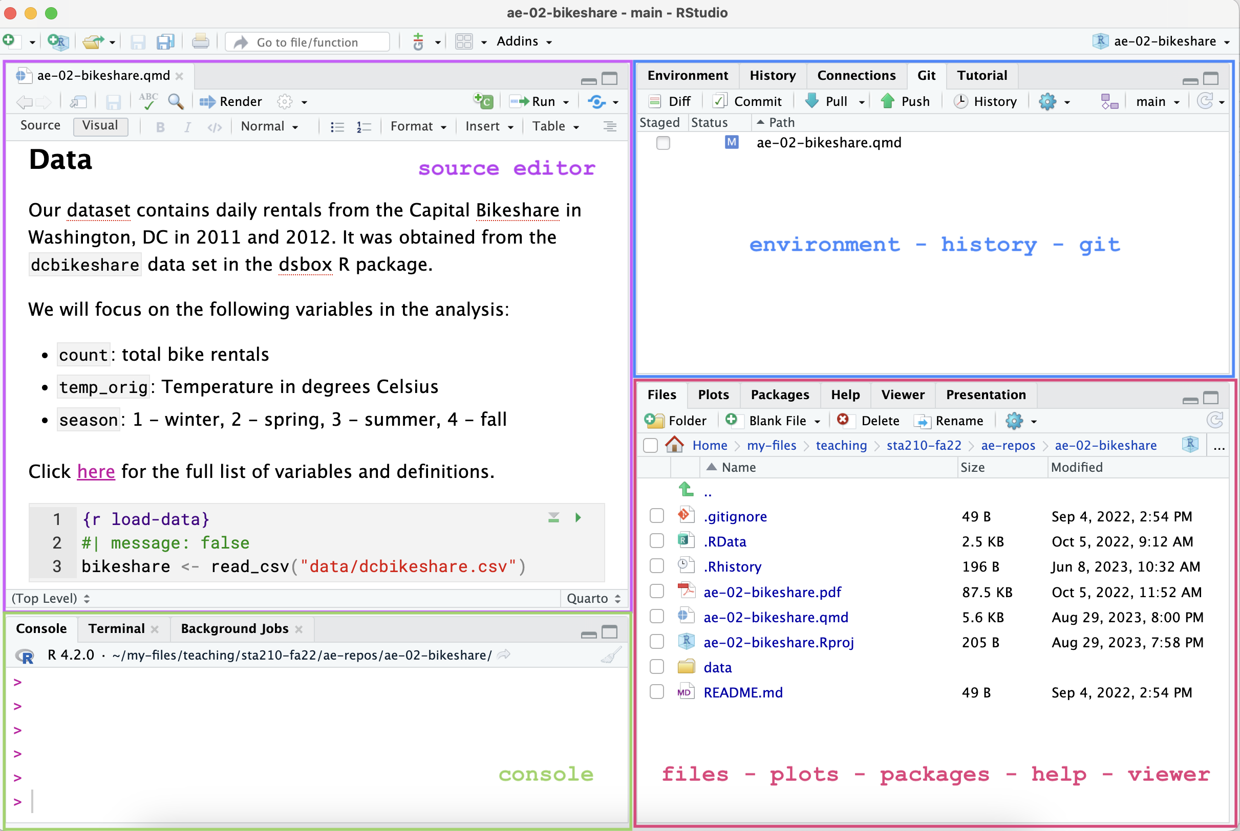
R and R Studio
Below are the components of the RStudio IDE.
Below are the components of an Quarto (.Rmd) file.
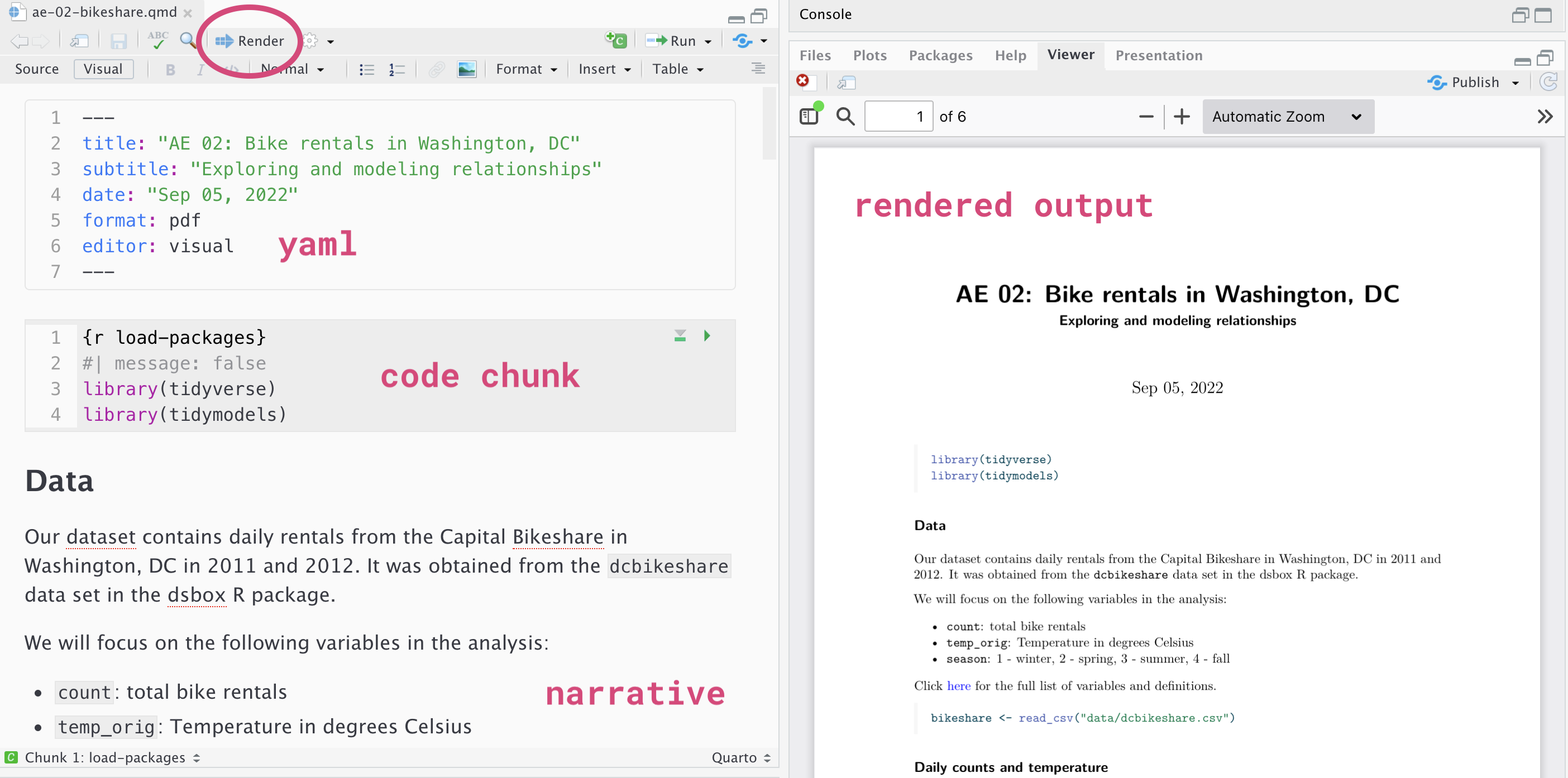
YAML
The top portion of your Quarto file (between the three dashed lines) is called YAML. It stands for “YAML Ain’t Markup Language”. It is a human friendly data serialization standard for all programming languages. All you need to know is that this area is called the YAML (we will refer to it as such) and that it contains meta information about your document.
Important
Open the Quarto (.qmd) file in your project, change the author name to your name, and render the document. Examine the rendered document.
Committing changes
Now, go to the Git pane in your RStudio instance. This will be in the top right hand corner in a separate tab.
If you have made changes to your Quarto (.qmd) file, you should see it listed here. Click on it to select it in this list and then click on Diff. This shows you the difference between the last committed state of the document and its current state including changes. You should see deletions in red and additions in green.
If you’re happy with these changes, we’ll prepare the changes to be pushed to your remote repository. First, stage your changes by checking the appropriate box on the files you want to prepare. Next, write a meaningful commit message (for instance, “updated author name”) in the Commit message box. Finally, click Commit. Note that every commit needs to have a commit message associated with it.
You don’t have to commit after every change, as this would get quite tedious. You should commit states that are meaningful to you for inspection, comparison, or restoration.
In the first few assignments we will tell you exactly when to commit and in some cases, what commit message to use. As the semester progresses we will let you make these decisions.
Now let’s make sure all the changes went to GitHub. Go to your GitHub repo and refresh the page. You should see your commit message next to the updated files. If you see this, all your changes are on GitHub and you’re good to go!
Push changes
Now that you have made an update and committed this change, it’s time to push these changes to your repo on GitHub.
In order to push your changes to GitHub, you must have staged your commit to be pushed. click on Push.
Packages
We will use the following packages in today’s lab.
library(tidyverse)
library(tidymodels)
library(skimr)
Data
Today’s data is about access to parks and other public amenities in the 100 most populated cities in the United States. The data were collected by the Trust for Public Land, a non-profit organization that advocates for equitable access to outdoor spaces. The data set we’ll use in this lab includes part of the data used for analysis in the 2021 special report Parks and Equitable Recovery; it was obtained from TidyTuesday.
Use the code below to load the data into R.
parks <- read_csv("data/parks.csv")This lab will focus on the following variables:
pct_near_park_points: Points in the Trust for Public Land ParkScore index for the percent of residents within a 10 minute walk to park points. Click here to learn more about the ParkScore.spend_per_resident_data: Spending per resident in US dollars.
Click here for the full data dictionary.
Exercises
Goal: One way to improve access to public parks is for cities to spend more money creating and maintaining parks for their residents. It’s unclear, however, how much spending impacts residents’ access to parks. The goal of this analysis is to examine the relationship between spending per resident and points in the ParkScore index for the percent of residents within a 10 minute walk to a park.
Write all code and narrative in your Quarto file. Write all narrative in complete sentences. Throughout the assignment, you should periodically render your Quarto document to produce the updated PDF, commit the changes in the Git pane, and push the updated files to GitHub.
Tip
Make sure we can read all of your code in your PDF document. This means you will need to break up long lines of code. One way to help avoid long lines of code is is start a new line after every pipe (|>) and plus sign (+).
Exercise 1
Viewing a summary of the data is a useful starting point for data analysis, especially if there are a large number of observations or variables. Run the code below to use the glimpse function to see a summary of the parks data frame.
How many observations (rows) are in parks? How many variables (columns)?
glimpse(parks)
Note
In your lab-01.qmd document you’ll see that we already added the code required for the exercise as well as a sentence where you can fill in the blanks to report the answer. Use this format for the remaining exercises.
Also note that the code chunk as a label: glimpse-data. It’s not required, but good practice and highly encouraged to label your code chunks using short meaningful names. (Hint: Do not uses spaces in code chunk labels. Use - to separate multiple words.)
Exercise 2
The predictor variable for this analysis spend_per_resident_data is quantitative; however, from the glimpse of the data in Exercise 1, we see its data type is chr (character) in R. We would expect it to be dbl (double), the data type for numeric data.
- Why did
spend_per_resident_dataget read by R as a character data type instead of a double? Be specific. - Why do we need to convert
spend_per_resident_datato a data type suitable for quantitative data? How might leaving it as a character variable hinder the analysis?
Exercise 3
Use the code below to convert spend_per_resident_data , so that it is correctly treated as quantitative data in R. Each line of code is numbered. Write a brief explanation of what each line of code does.
Tip
See Simple Linear Regression in R for an example of explaining code line by line.
1parks <- parks |>
  mutate(spend_per_resident_data =
2           str_replace(spend_per_resident_data,"\\$", "")) |>
  mutate(spend_per_resident_data =
3 as.numeric(spend_per_resident_data))- 1
- ______
- 2
- ______
- 3
- ______
This is a good place to render, commit, and push changes to your lab-01 repo on GitHub. Write an informative commit message (e.g. “Completed exercises 1 - 3”), and push every file to GitHub by clicking the checkbox next to each file in the Git pane. After you push the changes, the Git pane in RStudio should be empty.
Exercise 4
Exploratory data analysis (EDA) helps us “get to know” the data and examine the variable distributions and relationships between variables. We do so using visualizations and summary statistics.
When we make visualizations, we want them to be clear and suitable for a professional audience. This means that, at a minimum, each visualization should have an informative title and informative axis labels.
Fill in the code below to visualize the distribution of spend_per_resident_data using a histogram.
ggplot(data = ____, aes(x = ____)) +
  geom_histogram() +
    labs(x = "_____",
       y = "_____",
       title = "_____")
Then, fill in the code to calculate summary statistics for the variable using the skim function from the skimr R package (Waring et al. 2022).
parks |>
  skim(____) |>
  select(-skim_type, -skim_variable, -complete_rate,
         - numeric.hist) |> #remove these columns from output
  print(width = Inf) #print all columns
Exercise 5
Use the visualization and summary statistics from the previous exercise to describe the distribution of spend_per_resident_data. In your narrative, include a description of the shape, center, spread, and the presence of apparent outliers or other interesting features.
Tip
See Univariate EDA for an example.
Exercise 6
Now let’s look at the distribution of the response variable pct_near_park_points.
Visualize this distribution and calculate the summary statistics. The visualization should have an informative title and informative axis labels.
Use the visualization and summary statistics to describe the distribution of
pct_near_park_points. Recall from the previous exercise the components to include the description.
This is another good place to render, commit, and push changes to your lab-01 repo on GitHub. Write an informative commit message (e.g. “Completed exercises 4 - 6”), and push every file to GitHub by clicking the checkbox next to each file in the Git pane. After you push the changes, the Git pane in RStudio should be empty.
Exercise 7
The parks data set ranges from the year 2012 to 2020, so each row contains information about funding and public amenities for each city in a given year. Thus, there are multiple rows in parks for each city. We are going to summarize the data, so there is just one row per city. Fill in the code below to create a new data frame called parks_summary that contains the mean spending per resident and mean points in the ParkScore index for the percent of residents within a 10-minute walk to a park.
parks_summary <- ____ |>
  group_by(____) |>
  summarise(mean_spend = mean(____),
            mean_pts_near = ____)
How many rows are in parks_summary? How many columns?
Important
Use parks_summary for exercises 8 - 9.
Exercise 8
- Create a visualization of the relationship between
mean_spendandmean_pts_near, and calculate the correlation between the two variables. Include an informative title and informative axis labels on the visualization.
- Use the visualization and correlation to describe the relationship between the two variables. Include the shape, direction, strength, presence of potential outliers, and any other interesting features in the description.
Tip
See Bivariate EDA for an example.
This is a good place to render, commit, and push changes to your lab-01 repo on GitHub. Write an informative commit message (e.g. “Completed exercises 7- 8”), and push every file to GitHub by clicking the checkbox next to each file in the Git pane. After you push the changes, the Git pane in RStudio should be empty.
Exercise 9
Fit and display a linear regression model of the relationship between
mean_spendandmean_pts_near. Use the tidymodels (Kuhn and Wickham 2020) syntax and display the model in a tidy format.Interpret the slope in the context of the data.
Interpret the intercept in the context of the data. Is the interpretation useful in practice for this data? Briefly explain.
Exercise 10
Parks and an Equitable Recovery, a special report by Trust for Public Land, begins with the following conclusion from their analysis:
Our data shows major disparities in access to the outdoors. In the 100 most populated cities, neighborhoods where most residents identify as Black, Hispanic and Latinx, American Indian/Alaska Native or Asian American and Pacific Islander have access to an average of 44 percent less park acreage than predominantly white neighborhoods, and similar park space inequities exist in low-income neighborhoods across cities, highlighting the urgent need to center equity in park investment and planning.
Would it be possible to reproduce the analysis results that led to this conclusion given the data we have in parks.csv? If so, briefly describe the steps we might take to reproduce the analysis. If not, briefly describe the additional data we need in order to reproduce the analysis.
You’re done and ready to submit your work! render, commit, and push all remaining changes. You can use the commit message “Done with Lab 1!”, and make sure you have pushed all the files to GitHub (your Git pane in RStudio should be empty) and that all documents are updated in your repo on GitHub. The PDF document you submit to Gradescope should be identical to the one in your GitHub repo.
See the instructions below to submit your work on Gradescope.
Submission
In this class, we’ll be submitting PDF documents to Gradescope.
Warning
Before you wrap up the assignment, make sure all documents are updated on your GitHub repo. We will be checking these to make sure you have been practicing how to commit and push changes.
Remember – you must turn in a PDF file to the Gradescope page before the submission deadline for full credit.
To submit your assignment:
- Go to http://www.gradescope.comand click Log in in the top right corner.
- Click School Credentials ➡️ Duke NetID and log in using your NetID credentials.
- Click on the STA 210 course.
- Click on the assignment, and you’ll be prompted to submit it.
- Mark the pages associated with each exercise. All of the pages of your lab should be associated with at least one question (i.e., should be “checked”).
- Select the first page of your .PDF submission to be associated with the “Workflow & formatting” section.
Grading (50 pts)
| Component | Points |
|---|---|
| Ex 1 | 2 |
| Ex 2 | 4 |
| Ex 3 | 6 |
| Ex 4 | 4 |
| Ex 5 | 4 |
| Ex 6 | 6 |
| Ex 7 | 3 |
| Ex 8 | 6 |
| Ex 9 | 6 |
| Ex 10 | 4 |
| Workflow & formatting | 51 |
References
Kuhn, Max, and Hadley Wickham. 2020. “Tidymodels: A Collection of Packages for Modeling and Machine Learning Using Tidyverse Principles.” https://www.tidymodels.org.
Waring, Elin, Michael Quinn, Amelia McNamara, Eduardo Arino de la Rubia, Hao Zhu, and Shannon Ellis. 2022. “Skimr: Compact and Flexible Summaries of Data.” https://CRAN.R-project.org/package=skimr.
Footnotes
The “Workflow & formatting” grade is to assess the reproducible workflow and document format. This includes having at least 3 informative commit messages, a neatly organized document with readable code and your name and the date in the YAML.↩︎