AE 06: Conditions and model evaluation

Songs on Spotify

Important

Go to the course GitHub organization and locate your ae-06 repo to get started.

Render, commit, and push your responses to GitHub by the end of class. The responses are due in your GitHub repo no later than Saturday, September 23 at 11:59pm.

library(tidyverse)
library(tidymodels)
library(knitr)
library(patchwork) #arrange plots in a grid

Data

The data set for this assignment is a subset from the Spotify Songs Tidy Tuesday data set. The data were originally obtained from Spotify using the spotifyr R package.

It contains numerous characteristics for each song. You can see the full list of variables and definitions here. This analysis will focus specifically on the following variables:

variable	class	description
track_id	character	Song unique ID
track_name	character	Song Name
track_artist	character	Song Artist
track_popularity	double	Song Popularity (0-100) where higher is better
energy	double	Energy is a measure from 0.0 to 1.0 and represents a perceptual measure of intensity and activity. Typically, energetic tracks feel fast, loud, and noisy. For example, death metal has high energy, while a Bach prelude scores low on the scale. Perceptual features contributing to this attribute include dynamic range, perceived loudness, timbre, onset rate, and general entropy.
valence	double	A measure from 0.0 to 1.0 describing the musical positiveness conveyed by a track. Tracks with high valence sound more positive (e.g. happy, cheerful, euphoric), while tracks with low valence sound more negative (e.g. sad, depressed, angry).

spotify <- read_csv("data/spotify-popular.csv")

Are high energy songs more positive? To answer this question, we’ll analyze data on some of the most popular songs on Spotify, i.e. those with track_popularity >= 80. We’ll use linear regression to fit a model to predict a song’s positiveness (valence) based on its energy level (energy).

Below are plots as part of the exploratory data analysis.

p1 <- ggplot(data = spotify, aes(x = valence)) + 
  geom_histogram() + 
  labs(title = "Distribution of Valence", 
       subtitle = " for Popular songs on Spotify", 
       x = "Valence")

p2 <- ggplot(data = spotify, aes(x = energy)) + 
  geom_histogram() + 
  labs(title = "Distribution of Energy", 
       subtitle = "for Popular songs on Spotify", 
       x = "Energy")
p1 + p2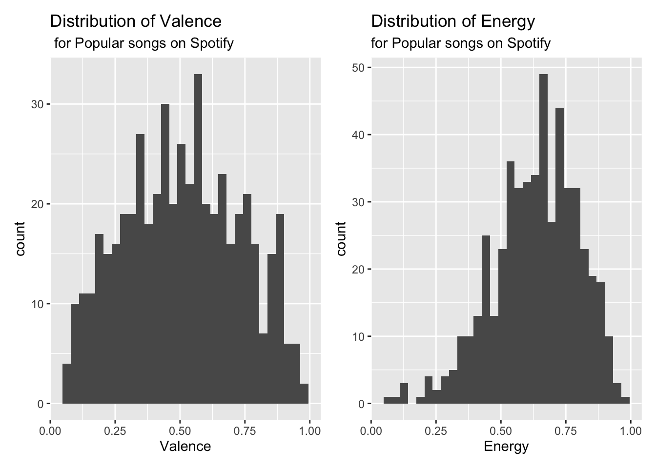

ggplot(data = spotify, aes(x = energy, y = valence)) + 
  geom_point() + 
  labs(title = "Valence vs. Energy", 
       subtitle = "Popular songs on Spotify", 
       x = "Energy", 
       y = "Valence")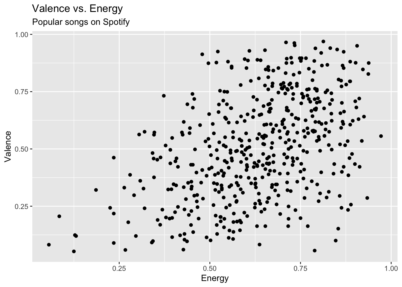

Exercise 1

Fit a model using the energy of a song to predict its valence, i.e. positiveness. Include the 90% confidence interval for the coefficients, and display the output using 3 digits.

## add code

Exercise 2

Let’s check the model conditions before doing any inference. Fill in the code below to use the augment() function to create a new data frame containing the residuals and fitted values (among other information)

Important

Note: Remove #|eval: false from the code chunk after you have filled in the code.

spotify_aug <- augment(_____)

Exercise 3

Make a plot of the residual vs. fitted values.

# add code here

Exercise 4

Fill in the code to make a histogram of the residuals and a normal QQ-plot.

resid_hist <- ggplot(data = ____, aes(x = ____)) +
  geom_histogram() +
  labs(x = "_____", 
       y = "_____", 
       title = "____")

resid_qq <- ggplot(data = ____, aes(sample = ____)) + 
  stat_qq() + 
 ____() + 
  labs(x = "_____", 
       y = "_____", 
       title = "____")

resid_hist + resid_qq

Exercise 5

Assess the four model conditions. Use the plots from the previous exercises to help make the assessment.

• Linearity
• Constant variance
• Normality
• Independence

Exercise 6

Calculate $R^2$ and interpret this value in the context of the data.

Exercise 7

Calculate RMSE and interpret this value in the context of the data.

Important

To submit the AE:

• Render the document to produce the PDF with all of your work from today’s class.
• Push all your work to your ae-06 repo on GitHub. (You do not submit AEs on Gradescope).