library(tidyverse)
library(tidymodels)
library(patchwork)AE 02: Bike rentals in Washington, DC
The big picture
Important
For this AE, you will discuss the questions in groups and submit answers on Ed Discussion. This AE does not count towards the Application Exercise grade.
Data
Our dataset contains daily rentals from the Capital Bikeshare in Washington, DC in 2011 and 2012. It was obtained from the dcbikeshare data set in the dsbox R package.
We will focus on the following variables in the analysis:
count: total bike rentalstemp_orig: Temperature in degrees Celsiusseason: 1 - winter, 2 - spring, 3 - summer, 4 - fall
Click here for the full list of variables and definitions.
bikeshare <- read_csv("data/dcbikeshare.csv")Daily counts and temperature
Exercise 1
Visualize the distribution of daily bike rentals and temperature as well as the relationship between these two variables.
p1 <- ggplot(bikeshare, aes(x = count)) +
  geom_histogram(binwidth = 250) +
  labs(x = "Daily bike rentals")

p2 <- ggplot(bikeshare, aes(x = temp_orig)) +
  geom_histogram() +
  labs(x = "Temperature (Celsius)")

p3 <- ggplot(bikeshare, aes(y = count, x = temp_orig)) +
  geom_point() +
  labs(x = "Temperature (Celsius)",
       y = "Daily bike rentals")

(p1 | p2) / p3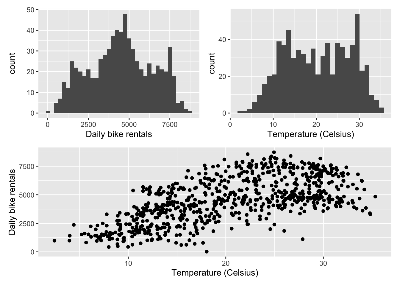
Exercise 2
Describe the relationship between daily bike rentals and temperature. Comment on how we expect the number of bike rentals to change as the temperature increases.
Exercise 3
Suppose you want to fit a model so you can use the temperature to predict the number of bike rentals. Would a model of the form
\[\text{count} = \beta_0 + \beta_1 ~ \text{temp\_orig} + \epsilon\]
be an appropriate fit for the data? Why or why not?
Put your group’s vote on Ed Discussion and briefly describe your reasoning in the comments.
Section 001 (10:05am): edstem.org/us/courses/44523/discussion/3361086
Section 002 (1:25pm): edstem.org/us/courses/44523/discussion/3361091