LR: Inference + conditions

Prof. Maria Tackett

Nov 13, 2023

Announcements

• Due dates

  • Draft report due in GitHub repo on 9am on the day of your lab

  • HW 04 due Wed, Nov 15 at 11:59pm

  • Statistics experience due Mon, Nov 20 at 11:59pm

• Next week:

  • (Optional) Project meetings Nov 20 & 21. Click here to sign up. Must sign up by Fri, Nov 17

  • No lecture Mon, Nov 20

  • No lab Tue, Nov 21

  • Thanksgiving Break: Wed, Nov 22 - Fri, Nov 24

Statistician of the day - Alejandra Castillo

Alejandra Castillo did her undergraduate work at Pomona College in Mathematics and her MS (2019) and PhD (2023) at Oregon State University in Statistics.

Dr. Castillo’s research lies at the intersection of unsupervised learning, dimension reduction, and inference, with applications in clinical trial design. Some of her work explores how to use baseline demographic information collected before randomization to a clinical trial, particularly as the baseline information changes during the course of the trial.

MS Thesis: Castillo A. On the Use of Baseline Values in Randomized Clinical Trials, MS Thesis, Oregon State, 2019.

Source: hardin47.github.io/CURV/scholars/castillo

Topics

• Estimating coefficients in logistic regression
• Inference for coefficients in logistic regression
• Checking model conditions for logistic regression

Computational setup

# load packages
library(tidyverse)
library(tidymodels)
library(openintro)
library(knitr)
library(kableExtra)  # for table embellishments
library(Stat2Data)   # for empirical logit

# set default theme and larger font size for ggplot2
ggplot2::theme_set(ggplot2::theme_bw(base_size = 20))

Data

Risk of coronary heart disease

This data set is from an ongoing cardiovascular study on residents of the town of Framingham, Massachusetts. We want to examine the relationship between various health characteristics and the risk of having heart disease.

• high_risk:

  • 1: High risk of having heart disease in next 10 years
  • 0: Not high risk of having heart disease in next 10 years

• age: Age at exam time (in years)

• education: 1 = Some High School, 2 = High School or GED, 3 = Some College or Vocational School, 4 = College

• currentSmoker: 0 = nonsmoker, 1 = smoker

Data prep

heart_disease <- read_csv(here::here("slides", "data/framingham.csv")) |>
  select(age, education, TenYearCHD, totChol, currentSmoker) |>
  drop_na() |>
  mutate(
    high_risk = as.factor(TenYearCHD),
    education = as.factor(education),
    currentSmoker = as.factor(currentSmoker)
  )

heart_disease

# A tibble: 4,086 × 6
     age education TenYearCHD totChol currentSmoker high_risk
   <dbl> <fct>          <dbl>   <dbl> <fct>         <fct>    
 1    39 4                  0     195 0             0        
 2    46 2                  0     250 0             0        
 3    48 1                  0     245 1             0        
 4    61 3                  1     225 1             1        
 5    46 3                  0     285 1             0        
 6    43 2                  0     228 0             0        
 7    63 1                  1     205 0             1        
 8    45 2                  0     313 1             0        
 9    52 1                  0     260 0             0        
10    43 1                  0     225 1             0        
# ℹ 4,076 more rows

Estimating coefficients

Statistical model

The form of the statistical model for logistic regression is

\[ \log\Big(\frac{\pi}{1-\pi}\Big) = \beta_0 + \beta_1X_1 + \beta_2X_2 + \dots + \beta_pX_p \]

where \(\pi\) is the probability \(Y = 1\).

Notice there is no error term when writing the statistical model for logistic regression. Why?

• Recall that the statistical model is the “data-generating” model
• Each individual observed \(Y\) is generated from a Bernoulli distribution, \(Bernoulli(\pi)\) (similarly we can think of \(n\) observed \(Y\)’s as generated from a Binomial distribution, \(Binomial(n,p)\))
• Therefore, the randomness is not produced by an error term but rather in the distribution used to generate \(Y\)

Estimating coefficients

Recall the log likelihood function

\[ \log L = \sum\limits_{i=1}^n[y_i \log(\hat{\pi}_i) + (1 - y_i)\log(1 - \hat{\pi}_i)] \]

where

\(\hat{\pi} = \frac{exp\{\hat{\beta}_0 + \hat{\beta}_1X_1 + \dots + \hat{\beta}_pX_p\}}{1 + exp\{\hat{\beta}_0 + \hat{\beta}_1X_1 + \dots + \hat{\beta}_pX_p\}}\)

• The coefficients \(\hat{\beta}_0, \ldots, \hat{\beta}_p\) are estimated using maximum likelihood estimation

• Basic idea: Find the values of \(\hat{\beta}_0, \ldots, \hat{\beta}_p\) that give the observed data the maximum probability of occurring

Application exercise

📋 AE 15: Inference for Logistic Regression

Inference for coefficients

Modeling risk of coronary heart disease

Using age and education:

risk_fit <- logistic_reg() |>
  set_engine("glm") |>
  fit(high_risk ~ age + education, 
      data = heart_disease, family = "binomial")

Model output

tidy(risk_fit, conf.int = TRUE) |> 
  kable(format = "markdown", digits = 3)

term	estimate	std.error	statistic	p.value	conf.low	conf.high
(Intercept)	-5.508	0.311	-17.692	0.000	-6.125	-4.904
age	0.076	0.006	13.648	0.000	0.065	0.087
education2	-0.245	0.113	-2.172	0.030	-0.469	-0.026
education3	-0.236	0.135	-1.753	0.080	-0.504	0.024
education4	-0.024	0.150	-0.161	0.872	-0.323	0.264

\[ \small{\log\Big(\frac{\hat{\pi}}{1-\hat{\pi}}\Big) = -5.508 + 0.076 ~ \text{age} - 0.245 ~ \text{ed2} - 0.236 ~ \text{ed3} - 0.024 ~ \text{ed4}} \]

Inference for coefficients

There are two approaches for testing coefficients in logistic regression

• Drop-in-deviance test. Use to test…

  • a single coefficient
  • a categorical predictor with 3+ levels
  • a group of predictor variables

• (Wald) hypothesis test. Use to test

  • a single coefficient

Hypothesis test for \(\beta_j\)

Hypotheses: \(H_0: \beta_j = 0 \hspace{2mm} \text{ vs } \hspace{2mm} H_a: \beta_j \neq 0\), given the other variables in the model

Test Statistic: \[z = \frac{\hat{\beta}_j - 0}{SE_{\hat{\beta}_j}}\]

P-value: \(P(|Z| > |z|)\), where \(Z \sim N(0, 1)\), the Standard Normal distribution

Confidence interval for \(\beta_j\)

We can calculate the C% confidence interval for \(\beta_j\) as the following:

\[ \Large{\hat{\beta}_j \pm z^* SE_{\hat{\beta}_j}} \]

where \(z^*\) is calculated from the \(N(0,1)\) distribution

Note

This is an interval for the change in the log-odds for every one unit increase in \(x_j\)

Interpretation in terms of the odds

The change in odds for every one unit increase in \(x_j\).

\[ \Large{exp\{\hat{\beta}_j \pm z^* SE_{\hat{\beta}_j}\}} \]

Interpretation: We are \(C\%\) confident that for every one unit increase in \(x_j\), the odds multiply by a factor of \(exp\{\hat{\beta}_j - z^* SE_{\hat{\beta}_j}\}\) to \(exp\{\hat{\beta}_j + z^* SE_{\hat{\beta}_j}\}\), holding all else constant.

Coefficient for age

term	estimate	std.error	statistic	p.value	conf.low	conf.high
(Intercept)	-5.508	0.311	-17.692	0.000	-6.125	-4.904
age	0.076	0.006	13.648	0.000	0.065	0.087
education2	-0.245	0.113	-2.172	0.030	-0.469	-0.026
education3	-0.236	0.135	-1.753	0.080	-0.504	0.024
education4	-0.024	0.150	-0.161	0.872	-0.323	0.264

Hypotheses:

\[ H_0: \beta_{age} = 0 \hspace{2mm} \text{ vs } \hspace{2mm} H_a: \beta_{age} \neq 0 \], given education is in the model

Coefficient for age

term	estimate	std.error	statistic	p.value	conf.low	conf.high
(Intercept)	-5.508	0.311	-17.692	0.000	-6.125	-4.904
age	0.076	0.006	13.648	0.000	0.065	0.087
education2	-0.245	0.113	-2.172	0.030	-0.469	-0.026
education3	-0.236	0.135	-1.753	0.080	-0.504	0.024
education4	-0.024	0.150	-0.161	0.872	-0.323	0.264

Test statistic:

\[z = \frac{0.07559 - 0}{0.00554} = 13.64 \]

Coefficient for age

term	estimate	std.error	statistic	p.value	conf.low	conf.high
(Intercept)	-5.508	0.311	-17.692	0.000	-6.125	-4.904
age	0.076	0.006	13.648	0.000	0.065	0.087
education2	-0.245	0.113	-2.172	0.030	-0.469	-0.026
education3	-0.236	0.135	-1.753	0.080	-0.504	0.024
education4	-0.024	0.150	-0.161	0.872	-0.323	0.264

P-value:

\[ P(|Z| > |13.64|) \approx 0 \]

2 * pnorm(13.64,lower.tail = FALSE)

[1] 2.315606e-42

Coefficient for age

term	estimate	std.error	statistic	p.value	conf.low	conf.high
(Intercept)	-5.508	0.311	-17.692	0.000	-6.125	-4.904
age	0.076	0.006	13.648	0.000	0.065	0.087
education2	-0.245	0.113	-2.172	0.030	-0.469	-0.026
education3	-0.236	0.135	-1.753	0.080	-0.504	0.024
education4	-0.024	0.150	-0.161	0.872	-0.323	0.264

Conclusion:

The p-value is very small, so we reject \(H_0\). The data provide sufficient evidence that age is a statistically significant predictor of whether someone is high risk of having heart disease, after accounting for education.

CI for age

term	estimate	std.error	statistic	p.value	conf.low	conf.high
(Intercept)	-5.508	0.311	-17.692	0.000	-6.125	-4.904
age	0.076	0.006	13.648	0.000	0.065	0.087
education2	-0.245	0.113	-2.172	0.030	-0.469	-0.026
education3	-0.236	0.135	-1.753	0.080	-0.504	0.024
education4	-0.024	0.150	-0.161	0.872	-0.323	0.264

Interpret the 95% confidence interval for age in terms of the odds of being high risk for heart disease.

Application exercise

📋 AE 15: Inference for Logistic Regression

Conditions

The model

Let’s predict high_risk from age, total cholesterol, and whether the patient is a current smoker:

risk_fit <- logistic_reg() |>
  set_engine("glm") |>
  fit(high_risk ~ age + totChol + currentSmoker, 
      data = heart_disease, family = "binomial")

tidy(risk_fit, conf.int = TRUE) |> 
  kable(digits = 3)

term	estimate	std.error	statistic	p.value	conf.low	conf.high
(Intercept)	-6.673	0.378	-17.647	0.000	-7.423	-5.940
age	0.082	0.006	14.344	0.000	0.071	0.094
totChol	0.002	0.001	1.940	0.052	0.000	0.004
currentSmoker1	0.443	0.094	4.733	0.000	0.260	0.627

Conditions for logistic regression

1. Linearity: The log-odds have a linear relationship with the predictors.

2. Randomness: The data were obtained from a random process

3. Independence: The observations are independent from one another.

Empirical logit

The empirical logit is the log of the observed odds:

\[ \text{logit}(\hat{p}) = \log\Big(\frac{\hat{p}}{1 - \hat{p}}\Big) = \log\Big(\frac{\# \text{Yes}}{\# \text{No}}\Big) \]

Calculating empirical logit (categorical predictor)

If the predictor is categorical, we can calculate the empirical logit for each level of the predictor.

heart_disease |>
  count(currentSmoker, high_risk) |>
  group_by(currentSmoker) |>
  mutate(prop = n/sum(n)) |>
  filter(high_risk == "1") |>
  mutate(emp_logit = log(prop/(1-prop)))

# A tibble: 2 × 5
# Groups:   currentSmoker [2]
  currentSmoker high_risk     n  prop emp_logit
  <fct>         <fct>     <int> <dbl>     <dbl>
1 0             1           301 0.145     -1.77
2 1             1           318 0.158     -1.67

Calculating empirical logit (quantitative predictor)

1. Divide the range of the predictor into intervals with approximately equal number of cases. (If you have enough observations, use 5 - 10 intervals.)

2. Compute the empirical logit for each interval

You can then calculate the mean value of the predictor in each interval and create a plot of the empirical logit versus the mean value of the predictor in each interval.

Empirical logit plot in R (quantitative predictor)

Created using dplyr and ggplot functions.

Empirical logit plot in R (quantitative predictor)

Created using dplyr and ggplot functions.

heart_disease |> 
  mutate(age_bin = cut_interval(age, n = 10)) |>
  group_by(age_bin) |>
  mutate(mean_age = mean(age)) |>
  count(mean_age, high_risk) |>
  mutate(prop = n/sum(n)) |>
  filter(high_risk == "1") |>
  mutate(emp_logit = log(prop/(1-prop))) |>
  ggplot(aes(x = mean_age, y = emp_logit)) + 
  geom_point() + 
  geom_smooth(method = "lm", se = FALSE) +
  labs(x = "Mean Age", 
       y = "Empirical logit")

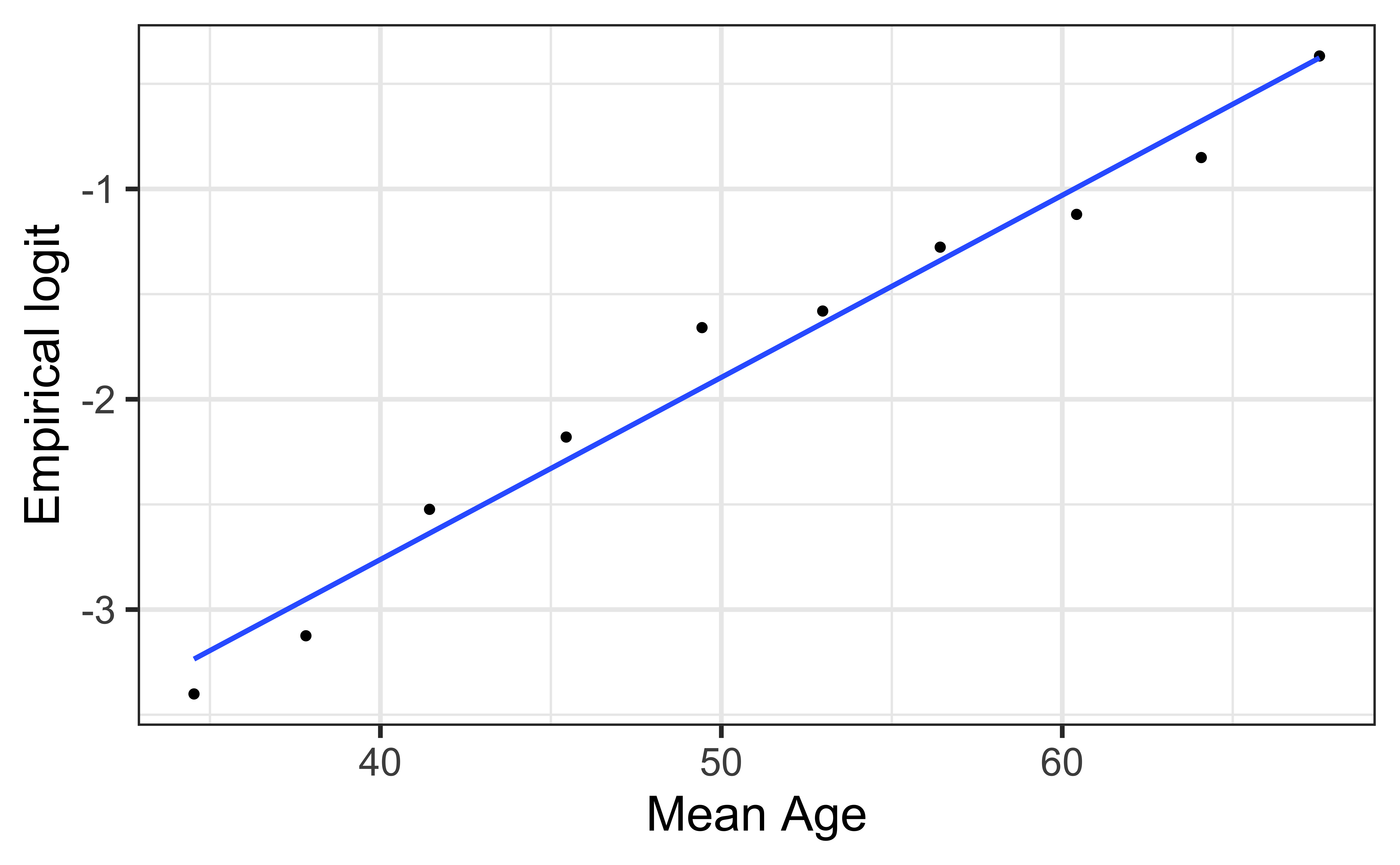
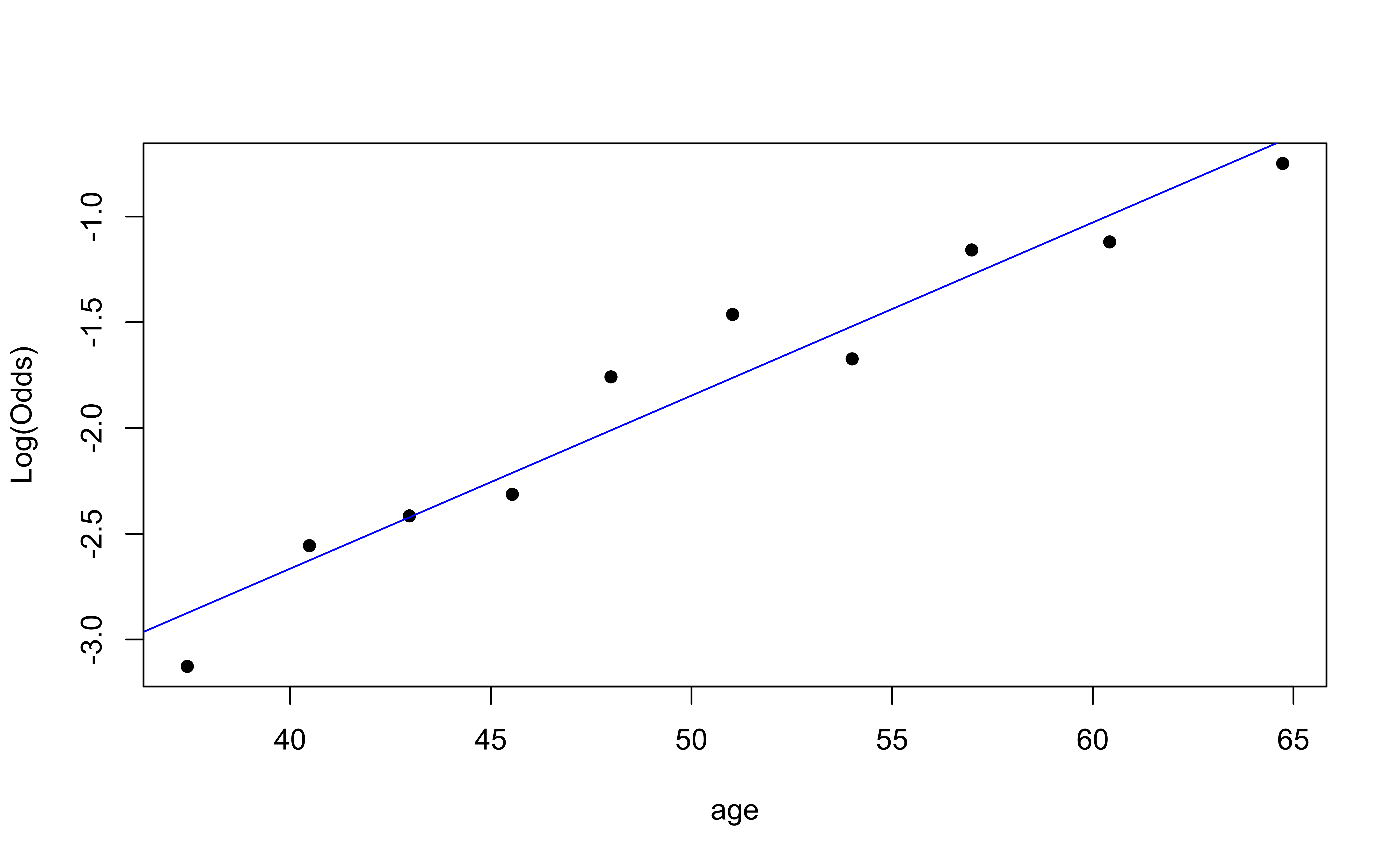
Empirical logit plot in R (quantitative predictor)

Using the emplogitplot1 function from the Stat2Data R package

emplogitplot1(high_risk ~ age, 
              data = heart_disease, 
              ngroups = 10)

Empirical logit plot in R (interactions)

Using the emplogitplot2 function from the Stat2Data R package

emplogitplot2(high_risk ~ age + currentSmoker, data = heart_disease, 
              ngroups = 10, 
              putlegend = "bottomright")

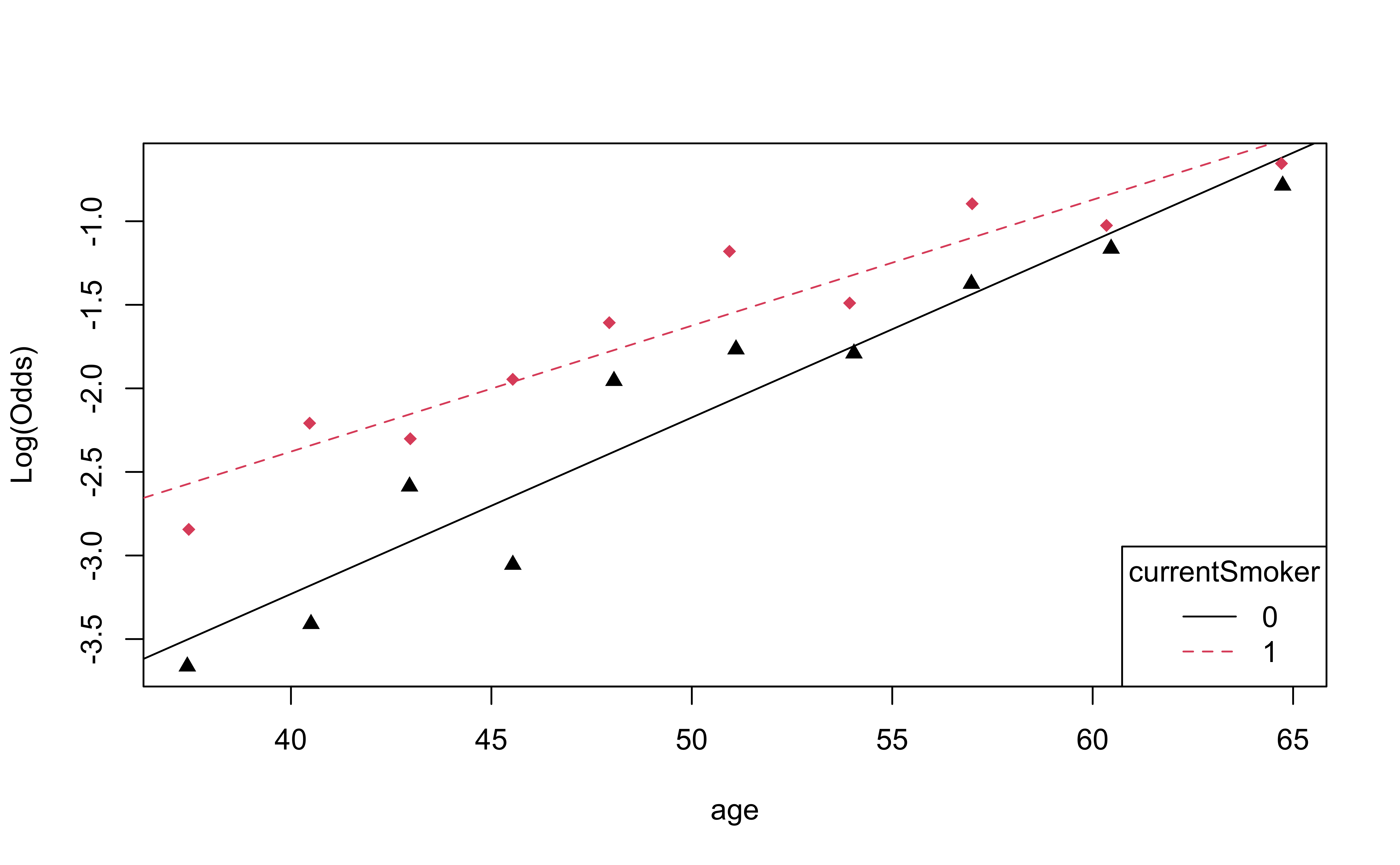
Checking linearity

emplogitplot1(high_risk ~ age, 
              data = heart_disease, 
              ngroups = 10)

emplogitplot1(high_risk ~ totChol, 
              data = heart_disease, 
              ngroups = 10)

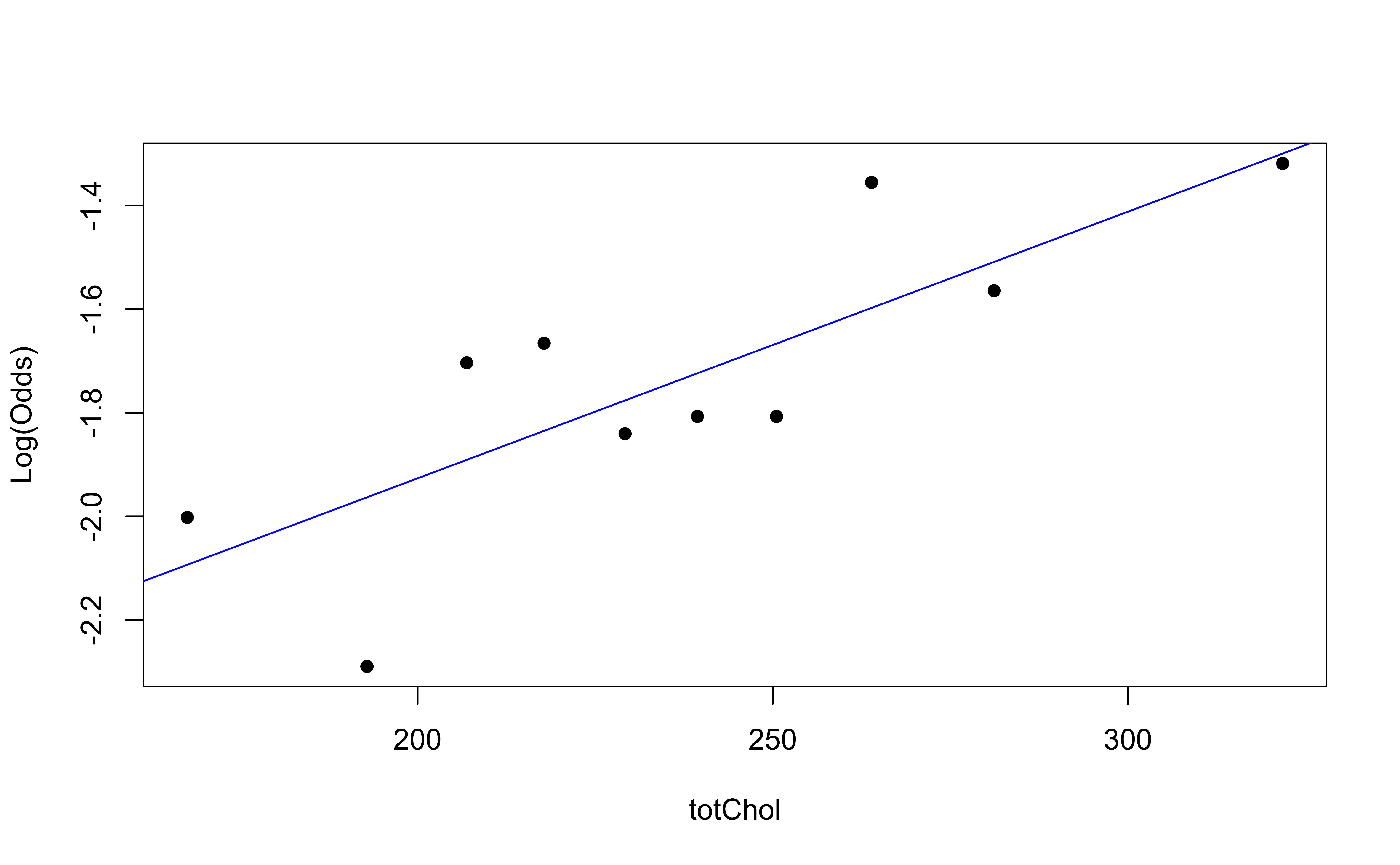
✅ The linearity condition is satisfied. There is a linear relationship between the empirical logit and the predictor variables.

Checking randomness

We can check the randomness condition based on the context of the data and how the observations were collected.

• Was the sample randomly selected?
• If the sample was not randomly selected, ask whether there is reason to believe the observations in the sample differ systematically from the population of interest.

✅ The randomness condition is satisfied. We do not have reason to believe that the participants in this study differ systematically from adults in the U.S. in regards to health characteristics and risk of heart disease.

Checking independence

• We can check the independence condition based on the context of the data and how the observations were collected.
• Independence is most often violated if the data were collected over time or there is a strong spatial relationship between the observations.

✅ The independence condition is satisfied. It is reasonable to conclude that the participants’ health characteristics are independent of one another.