library(tidyverse)
library(tidymodels)
library(knitr)AE 15: Inference for logistic regression
Important
Go to the course GitHub organization and locate your ae-15 repo to get started.Render, commit, and push your responses to GitHub by the end of class.
The responses are due in your GitHub repo no later than Thursday, November 16 at 11:59pm.
Packages
Response to Leukemia treatment
Today’s data is from a study where 51 untreated adult patients with Acute Myeloid Leukemia who were given a course of treatment, and they were assessed as to their response to the treatment.1
The goal of today’s analysis is to use pre-treatment factors to predict how likely it is a patient will respond to the treatment.
We will use the following variables:
Age: Age at diagnosis (in years)Smear: Differential percentage of blastsInfil: Percentage of absolute marrow leukemia infiltrateIndex: Percentage labeling index of the bone marrow leukemia cellsBlasts: Absolute number of blasts, in thousandsTemp: Highest temperature of the patient prior to treatment, in degrees FahrenheitResp: 1 = responded to treatment or 0 = failed to respond
leukemia <- read_csv("data/leukemia.csv") |>
  mutate(Resp = factor(Resp))
Estimating coefficients for logistic regression
Illustrating maximum likelihood estimation (MLE)
Suppose we want to use the data to understand the probability a randomly selected adult diagnosed with leukemia will respond to the treatment.
Here are the results from our data:
leukemia %>%
  count(Resp) %>%
  mutate(prob = n /sum(n))
# A tibble: 2 × 3
Resp n prob
<fct> <int> <dbl>
1 0 27 0.529
2 1 24 0.471Let’s set up some notation:
- \(Y\): Bernoulli random variable indicating whether an adult diagnosed with leukemia responds to the treatment
- \(y_i\): outcome for an individual adult (1: responded to treatment or 0: failed to respond)
- \(p\): probability a randomly selected adult diagnosed with leukemia responds to the treatment
Our goal is to find the most likely value of \(p\) given our data.
The likelihood function of the outcome for a single randomly selected adult diagnosed with leukemia is \[P(Y = y_i) = p^{y_i}(1-p)^{1-y_i}\]
The likelihood function, i.e. the joint probability, for the outcomes of 51 adults is
\[L = P(y_1, y_2, \ldots, y_{51}) = \prod_{i = 1}^{51} p^{y_i} (1 - p)^{1 - y_i}\]
We often use the log of the likelihood function, so we can work with sums rather than products.
\[\begin{aligned}\log L = \log[P(y_1, y_2, \ldots, y_{51})] &= \log\Big[\prod_{i = 1}^{51} p^{y_i} (1 - p)^{1 - y_i}\Big] \\ &= \sum_{i=1}^{51} y_i \log(p) + (1 - y_i)\log(1 - p)\end{aligned}\]
We can rewrite the equation and plug in the results from our data:
\[\begin{aligned} \log L &= \sum_{i=1}^{51} y_i \log(p) + (1 - y_i)\log(1 - p) \\ & = \log(p)\sum_{i=1}^{51}y_i + \log(1 - p)\sum_{i=1}^{51}(1 - y_{i}) \\ & = \log(p)\times 24 + \log(1 - p)\times 27 \end{aligned}\]
Let’s plug in different values of \(p\) and find the value that maximizes this equation.
p <- seq(0.01,.99,0.005)
logL <- log(p)*24+ log(1-p)*27 #log likelihood
L <- exp(logL) #likelihood
results <- tibble(p, logL, L)

#identify the the mle
results <- results %>%
  mutate(mle = if_else(logL == max(results$logL), "1", "0"))
# plot log likelihood
ggplot(data = results, aes(x = p, y = logL)) +
geom_point(aes(color = mle)) +
geom_line() +
scale_color_manual(values = c("gray", "red")) +
scale_x_continuous(breaks = seq(0,1,.1)) +
labs(title = "Maximizing Log Liklehood") 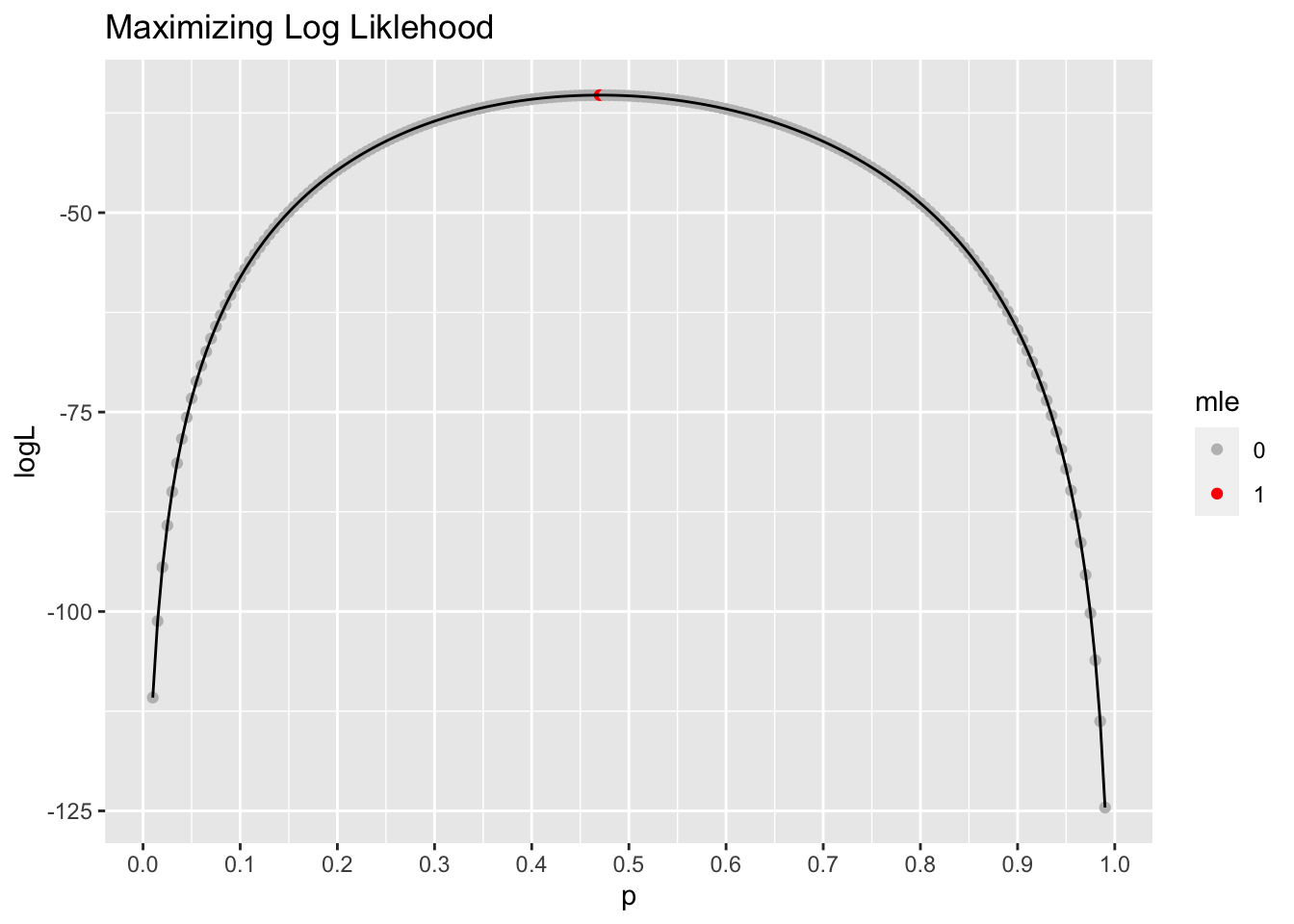
#plot likelihood
ggplot(data = results, aes(x = p, y = L)) +
  geom_point(aes(color = mle)) +
  geom_line() +
  scale_color_manual(values = c("gray", "red")) +
  scale_x_continuous(breaks = seq(0,1,.1)) +
labs(title = "Maximizing Likelihood") 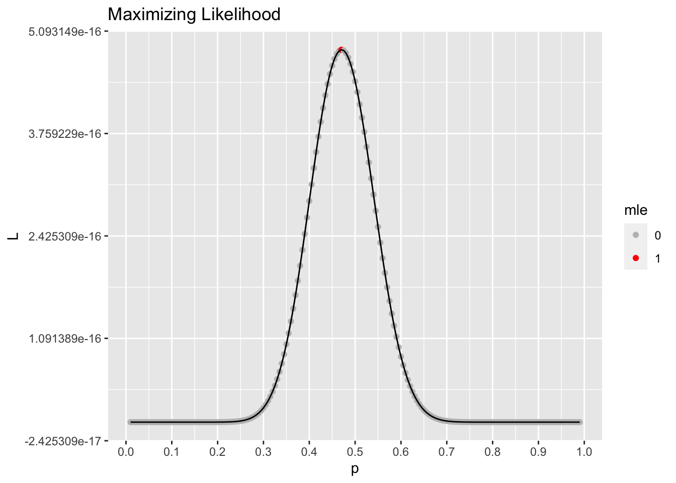
The MLE, the value that maximizes the (log) likelihood function is
results %>%
  filter(mle == 1)
# A tibble: 1 × 4
p logL L mle
<dbl> <dbl> <dbl> <chr>
1 0.47 -35.3 4.85e-16 1 As we might expect, this is the sample proportion \(\hat{p}\) from our data.
Extending to logistic regression
The parameters for logistic regression are estimated using maximum likelihood estimation. Suppose we have the model
\[\log\big(\frac{\pi}{1-\pi}\big) = \beta_0 + \beta_1 x\]
The estimates \(\hat{\beta}_0\) and \(\hat{\beta}_1\) are the ones maximize the log likelihood function
\[L = P(y_1, y_2, \ldots, y_n) = \prod_{i = 1}^{n} \pi^{y_i}(1-\pi)^{1-y_i}\]
where \[\pi = \frac{\exp\{\beta_0 + \beta_1x\}}{1 + \exp\{\beta_0 + \beta_1x\}}\]
There isn’t a closed-form solution for the log-likelihood, so numerical methods such as Iterative Weighted Least Squares are used to estimate the coefficients (learn more about IWLS in STA 211 and STA 310). This is the method used to estimate the coefficients in R.
Let’s fit a model using Age as a predictor and see some details of coefficient estimation.2 This is for demonstration purposes.
# Function that allows us to see the coefficients at each iteration
trace(glm.fit, quote(cat <- function(...) {
  base::cat(...)
  if (...length() >= 3 && identical(..3, " Iterations - ")) print(coefold)
}))
[1] "glm.fit"# Fit model to see details
resp_fit_details <- glm(Resp ~ Age, data = leukemia,
family = "binomial",
control = glm.control(trace = TRUE))Tracing glm.fit(x = structure(c(1, 1, 1, 1, 1, 1, 1, 1, 1, 1, 1, 1, 1, .... on entry
Deviance = 64.07455 Iterations - 1
NULL
Deviance = 64.0038 Iterations - 2
[1] 2.44957126 -0.05199527
Deviance = 64.00374 Iterations - 3
[1] 2.18965178 -0.04660907
Deviance = 64.00374 Iterations - 4
[1] 2.196772 -0.046760untrace(glm.fit)Final model
resp_fit <- logistic_reg() |>
  fit(Resp ~ Age, data = leukemia, family = "binomial")

tidy(resp_fit)
# A tibble: 2 × 5
term estimate std.error statistic p.value
<chr> <dbl> <dbl> <dbl> <dbl>
1 (Intercept) 2.20 1.01 2.18 0.0289
2 Age -0.0468 0.0195 -2.39 0.0166Inference for coefficients
- Fit a model using
Temp,Age, andIndexto predict whether or not a patient responds to the treatment. Display the model and the 95% confidence interval for the model coefficients.
# add code hereInterpret the coefficient of
Tempin the context of the data in terms of the odds an individual responds to the treatment.Interpret the 95% confidence interval for the coefficient of
Tempin terms of the odds an individual responds to the treatment.What is the distribution of the test statistic associated with
Temp?Is
Tempa useful predictor of the likelihood an individual responds to the treatment? Briefly explain.
Submission
Important
To submit the AE:
- Render the document to produce the PDF with all of your work from today’s class.
- Push all your work to your
ae-15repo on GitHub. (You do not submit AEs on Gradescope).
Footnotes
The data set is from the Stat2Data R package. This AE is adapted from exercises in Stat 2.↩︎
Trace function for current version of R from StackOverflow.↩︎