Logistic Regression: Prediction + classification

Prof. Maria Tackett

Nov 06, 2023

Announcements

• Lab this week: Work on project

• Project draft due in your GitHub repo at 9am on

  • November 14 (Tuesday labs)

  • November 16 (Thursday labs)

  • Will do peer review in lab those days

• Team Feedback #1 due Friday, November 10 at 11:5pm

  • Will receive email from Teammates

Odds ratios practice

Let’s take a look at one of the models from Lab 06 using flipper length and species to predict the odds a penguin is large (has a body mass above average).

term	estimate	std.error	statistic	p.value
(Intercept)	-39.151	7.149	-5.477	0.000
speciesChinstrap	-1.870	0.580	-3.221	0.001
speciesGentoo	0.512	0.843	0.607	0.544
flipper_length_mm	0.195	0.037	5.295	0.000

• Interpret the coefficient of flipper_length_mm in terms of the odds a penguin is large.

• Interpret the coefficient of speciesChinstrap in terms of the odds a penguin is large.

03:00

Topics

• Building predictive logistic regression models
• Sensitivity and specificity
• Making classification decisions

Computational setup

# load packages
library(tidyverse)
library(tidymodels)
library(openintro)
library(knitr)

# set default theme and larger font size for ggplot2
ggplot2::theme_set(ggplot2::theme_bw(base_size = 20))

Data

openintro::email

These data represent incoming emails for the first three months of 2012 for an email account.

• Outcome: spam - Indicator for whether the email was spam.
• Predictors: spam, to_multiple, from, cc, sent_email, time, image, attach, dollar, winner, inherit, viagra, password, num_char, line_breaks, format, re_subj, exclaim_subj, urgent_subj, exclaim_mess, number.

Click here for more detailed information on the variables.

Training and testing split

# Fix random numbers by setting the seed 
# Enables analysis to be reproducible when random numbers are used 
set.seed(1109)

# Put 75% of the data into the training set 
email_split <- initial_split(email)

# Create data frames for the two sets
email_train <- training(email_split)
email_test  <- testing(email_split)

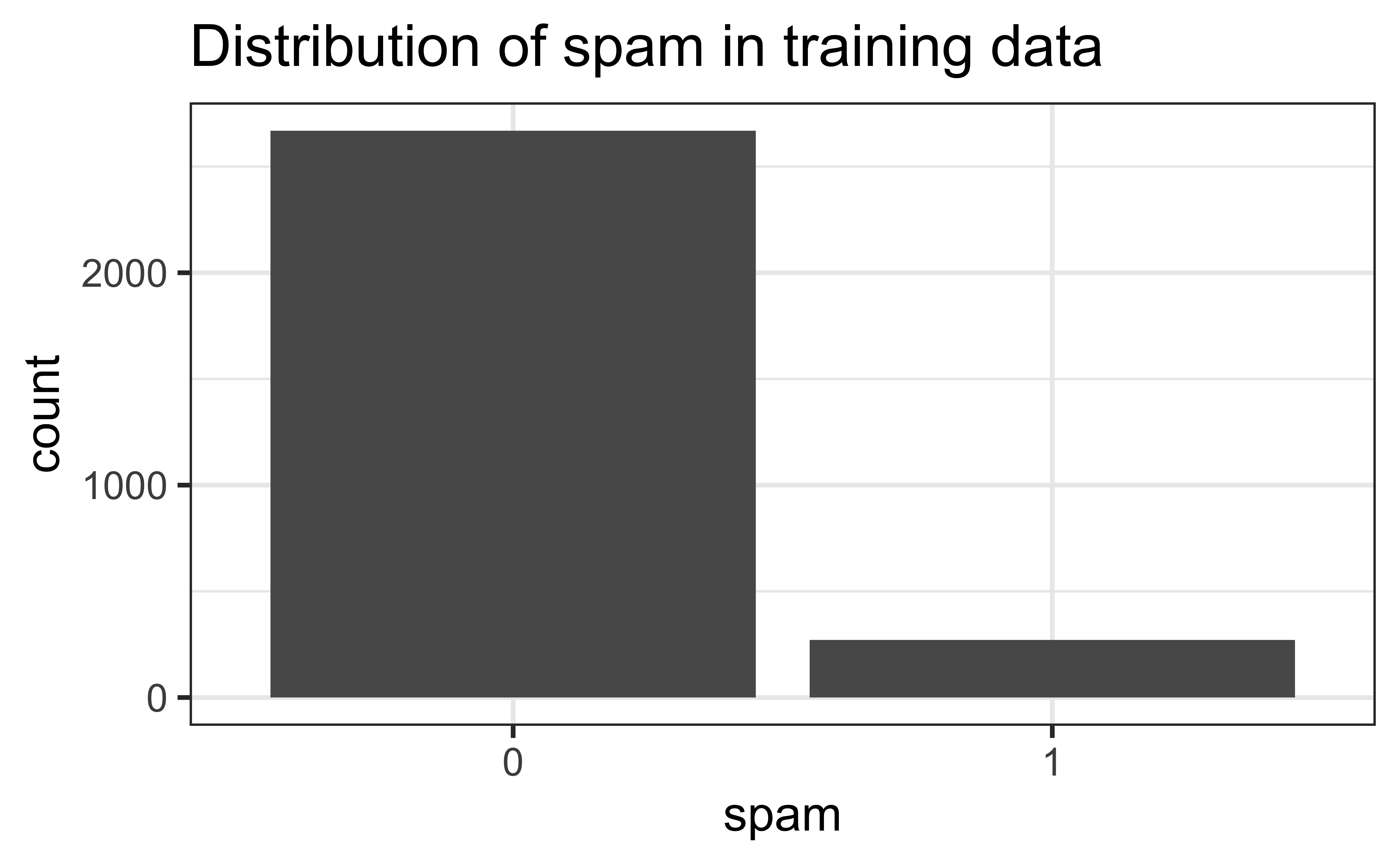
Exploratory data analysis

The sample is unbalanced with respect to spam.

Reminder: Modeling workflow

• Create a recipe for feature engineering steps to be applied to the training data

• Fit the model to the training data after these steps have been applied

  • Use cross-validation if deciding between multiple models

• Using the model estimates from the training data, predict outcomes for the test data

• Evaluate the performance of the model on the test data

Start with a recipe

Initiate a recipe

email_rec <- recipe(
  spam ~ .,          # formula
  data = email_train  # data to use for cataloging names and types of variables
  )
summary(email_rec)

# A tibble: 21 × 4
   variable     type      role      source  
   <chr>        <list>    <chr>     <chr>   
 1 to_multiple  <chr [3]> predictor original
 2 from         <chr [3]> predictor original
 3 cc           <chr [2]> predictor original
 4 sent_email   <chr [3]> predictor original
 5 time         <chr [1]> predictor original
 6 image        <chr [2]> predictor original
 7 attach       <chr [2]> predictor original
 8 dollar       <chr [2]> predictor original
 9 winner       <chr [3]> predictor original
10 inherit      <chr [2]> predictor original
11 viagra       <chr [2]> predictor original
12 password     <chr [2]> predictor original
13 num_char     <chr [2]> predictor original
14 line_breaks  <chr [2]> predictor original
15 format       <chr [3]> predictor original
16 re_subj      <chr [3]> predictor original
17 exclaim_subj <chr [2]> predictor original
18 urgent_subj  <chr [3]> predictor original
19 exclaim_mess <chr [2]> predictor original
20 number       <chr [3]> predictor original
21 spam         <chr [3]> outcome   original

Remove certain variables

email_rec <- email_rec |>
  step_rm(from, sent_email)

Feature engineer date

email_rec <- email_rec |>
  step_date(time, features = c("dow", "month")) |>
  step_rm(time)

Discretize numeric variables

email_rec <- email_rec |>
  step_cut(cc, attach, dollar, breaks = c(0, 1))

Create dummy variables

email_rec <- email_rec |>
  step_dummy(all_nominal(), -all_outcomes())

Remove zero variance variables

Variables that contain only a single value

email_rec <- email_rec |>
  step_zv(all_predictors())

Recipe: All in one place

email_rec <- recipe(spam ~ ., data = email_train) |>
  step_rm(from, sent_email) |>
  step_date(time, features = c("dow", "month")) |>               
  step_rm(time) |>
  step_cut(cc, attach, dollar, breaks = c(0, 1)) |>
  step_dummy(all_nominal_predictors()) |>
  step_zv(all_predictors())

Build a workflow

Define model

email_spec <- logistic_reg() |> 
  set_engine("glm")
email_spec

Logistic Regression Model Specification (classification)

Computational engine: glm 

Define workflow

Remember: Workflows bring together models and recipes so that they can be easily applied to both the training and test data.

email_wflow <- workflow() |> 
  add_model(email_spec) |> 
  add_recipe(email_rec)

══ Workflow ════════════════════════════════════════════════════════════════════
Preprocessor: Recipe
Model: logistic_reg()

── Preprocessor ────────────────────────────────────────────────────────────────
6 Recipe Steps

• step_rm()
• step_date()
• step_rm()
• step_cut()
• step_dummy()
• step_zv()

── Model ───────────────────────────────────────────────────────────────────────
Logistic Regression Model Specification (classification)

Computational engine: glm 

Fit model to training data

email_fit <- email_wflow |> 
  fit(data = email_train)

tidy(email_fit) |> print(n = 31)

# A tibble: 27 × 5
   term           estimate std.error statistic  p.value
   <chr>             <dbl>     <dbl>     <dbl>    <dbl>
 1 (Intercept)    -1.24      0.274     -4.51   6.43e- 6
 2 image          -1.36      0.679     -2.00   4.59e- 2
 3 inherit         0.352     0.185      1.90   5.69e- 2
 4 viagra          1.96     40.6        0.0482 9.62e- 1
 5 password       -0.941     0.387     -2.43   1.51e- 2
 6 num_char        0.0572    0.0257     2.23   2.58e- 2
 7 line_breaks    -0.00554   0.00147   -3.77   1.66e- 4
 8 exclaim_subj   -0.245     0.303     -0.807  4.19e- 1
 9 exclaim_mess    0.00916   0.00195    4.69   2.67e- 6
10 to_multiple_X1 -2.91      0.388     -7.50   6.37e-14
11 cc_X.1.68.     -0.105     0.446     -0.236  8.14e- 1
12 attach_X.1.21.  2.33      0.385      6.06   1.37e- 9
13 dollar_X.1.64.  0.0136    0.241      0.0565 9.55e- 1
14 winner_yes      2.46      0.480      5.12   3.02e- 7
15 format_X1      -1.02      0.173     -5.88   4.07e- 9
16 re_subj_X1     -2.93      0.436     -6.72   1.81e-11
17 urgent_subj_X1  4.37      1.25       3.51   4.54e- 4
18 number_small   -0.728     0.178     -4.08   4.45e- 5
19 number_big      0.261     0.255      1.03   3.05e- 1
20 time_dow_Mon    0.123     0.320      0.386  7.00e- 1
21 time_dow_Tue    0.309     0.294      1.05   2.94e- 1
22 time_dow_Wed   -0.133     0.297     -0.447  6.55e- 1
23 time_dow_Thu    0.104     0.303      0.343  7.32e- 1
24 time_dow_Fri    0.280     0.292      0.960  3.37e- 1
25 time_dow_Sat    0.439     0.323      1.36   1.74e- 1
26 time_month_Feb  1.06      0.192      5.54   3.06e- 8
27 time_month_Mar  0.575     0.198      2.91   3.60e- 3

Make predictions

Make predictions for test data

email_pred <- predict(email_fit, email_test, type = "prob") |> 
  bind_cols(email_test) 
email_pred

# A tibble: 981 × 23
   .pred_0  .pred_1 spam  to_multiple from     cc sent_email time               
     <dbl>    <dbl> <fct> <fct>       <fct> <int> <fct>      <dttm>             
 1   0.921 0.0786   0     0           1         0 0          2012-01-01 01:16:41
 2   0.961 0.0391   0     0           1         0 0          2012-01-01 05:00:01
 3   0.999 0.000988 0     0           1         1 1          2012-01-01 14:38:32
 4   0.999 0.000591 0     0           1         1 1          2012-01-01 18:40:14
 5   0.991 0.00878  0     0           1         0 0          2012-01-02 00:42:16
 6   0.910 0.0902   0     0           1         0 0          2012-01-01 21:05:45
 7   1.00  0.000108 0     1           1         3 0          2012-01-02 08:41:11
 8   0.975 0.0248   0     0           1         0 0          2012-01-02 20:07:17
 9   0.952 0.0477   0     0           1         0 0          2012-01-02 23:31:03
10   0.992 0.00819  0     1           1         0 0          2012-01-03 08:36:16
# ℹ 971 more rows
# ℹ 15 more variables: image <dbl>, attach <dbl>, dollar <dbl>, winner <fct>,
#   inherit <dbl>, viagra <dbl>, password <dbl>, num_char <dbl>,
#   line_breaks <int>, format <fct>, re_subj <fct>, exclaim_subj <dbl>,
#   urgent_subj <fct>, exclaim_mess <dbl>, number <fct>

A closer look at predictions

Which of the following 10 emails will be misclassified?

email_pred |>
  arrange(desc(.pred_1)) |>
  select(contains("pred"), spam) |> slice(1:10)

# A tibble: 10 × 3
   .pred_0 .pred_1 spam 
     <dbl>   <dbl> <fct>
 1  0.0750   0.925 0    
 2  0.110    0.890 0    
 3  0.116    0.884 1    
 4  0.127    0.873 1    
 5  0.170    0.830 1    
 6  0.189    0.811 1    
 7  0.204    0.796 1    
 8  0.208    0.792 1    
 9  0.224    0.776 1    
10  0.295    0.705 1    

Sensitivity and specificity

False positive and negative

	Email is spam	Email is not spam
Email classified as spam	True positive	False positive (Type 1 error)
Email classified as not spam	False negative (Type 2 error)	True negative

• False negative rate = P(classified as not spam | Email spam)

= FN / (TP + FN)

• False positive rate = P(classified as spam | Email not spam)

= FP / (FP + TN)

Sensitivity and specificity

	Email is spam	Email is not spam
Email classified as spam	True positive	False positive (Type 1 error)
Email classified as not spam	False negative (Type 2 error)	True negative

• Sensitivity = P(classified as spam | Email spam) = TP / (TP + FN)
  • Sensitivity = 1 − False negative rate
• Specificity = P(classified as not spam | Email not spam) = TN / (FP + TN)
  • Specificity = 1 − False positive rate

If you were designing a spam filter, would you want sensitivity and specificity to be high or low? What are the trade-offs associated with each decision?

Evaluate the performance

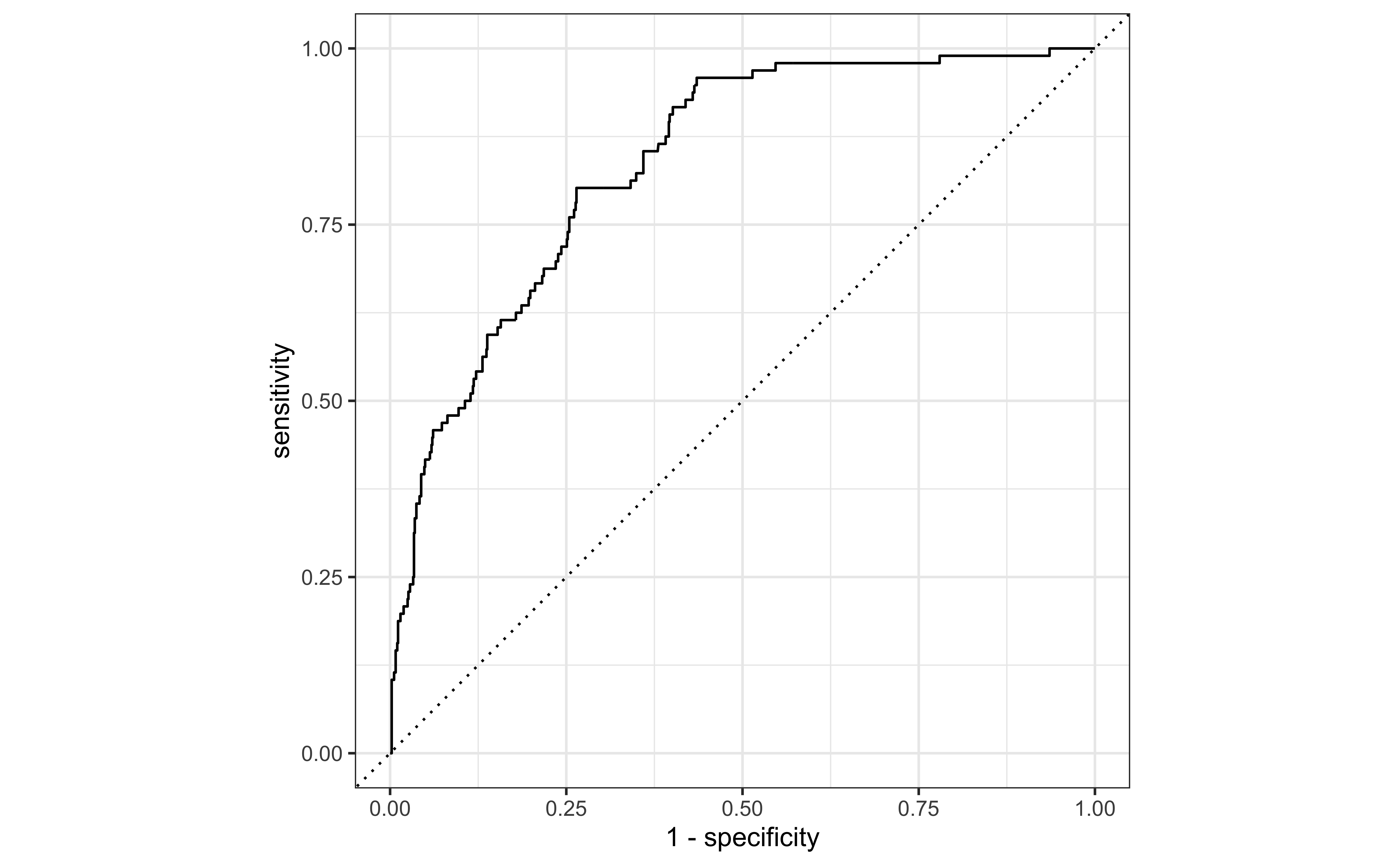
Receiver operating characteristic (ROC) curve⁺ plots the true positive rate (sensitivity) vs. false positive rate (1 - specificity).

email_pred |>
  roc_curve(
    truth = spam,
    .pred_1,
    event_level = "second"
  ) |>
  autoplot()

⁺ Originally developed for operators of military radar receivers, hence the name.

ROC curve, under the hood

email_pred |>
  roc_curve(
    truth = spam,
    .pred_1,
    event_level = "second"
  )

# A tibble: 978 × 3
    .threshold specificity sensitivity
         <dbl>       <dbl>       <dbl>
 1 -Inf            0                 1
 2    3.36e-10     0                 1
 3    2.27e- 9     0.00226           1
 4    8.69e- 7     0.00339           1
 5    9.89e- 7     0.00452           1
 6    1.43e- 6     0.00565           1
 7    9.16e- 6     0.00678           1
 8    1.03e- 5     0.00791           1
 9    2.58e- 5     0.00904           1
10    3.35e- 5     0.0102            1
# ℹ 968 more rows

ROC curve

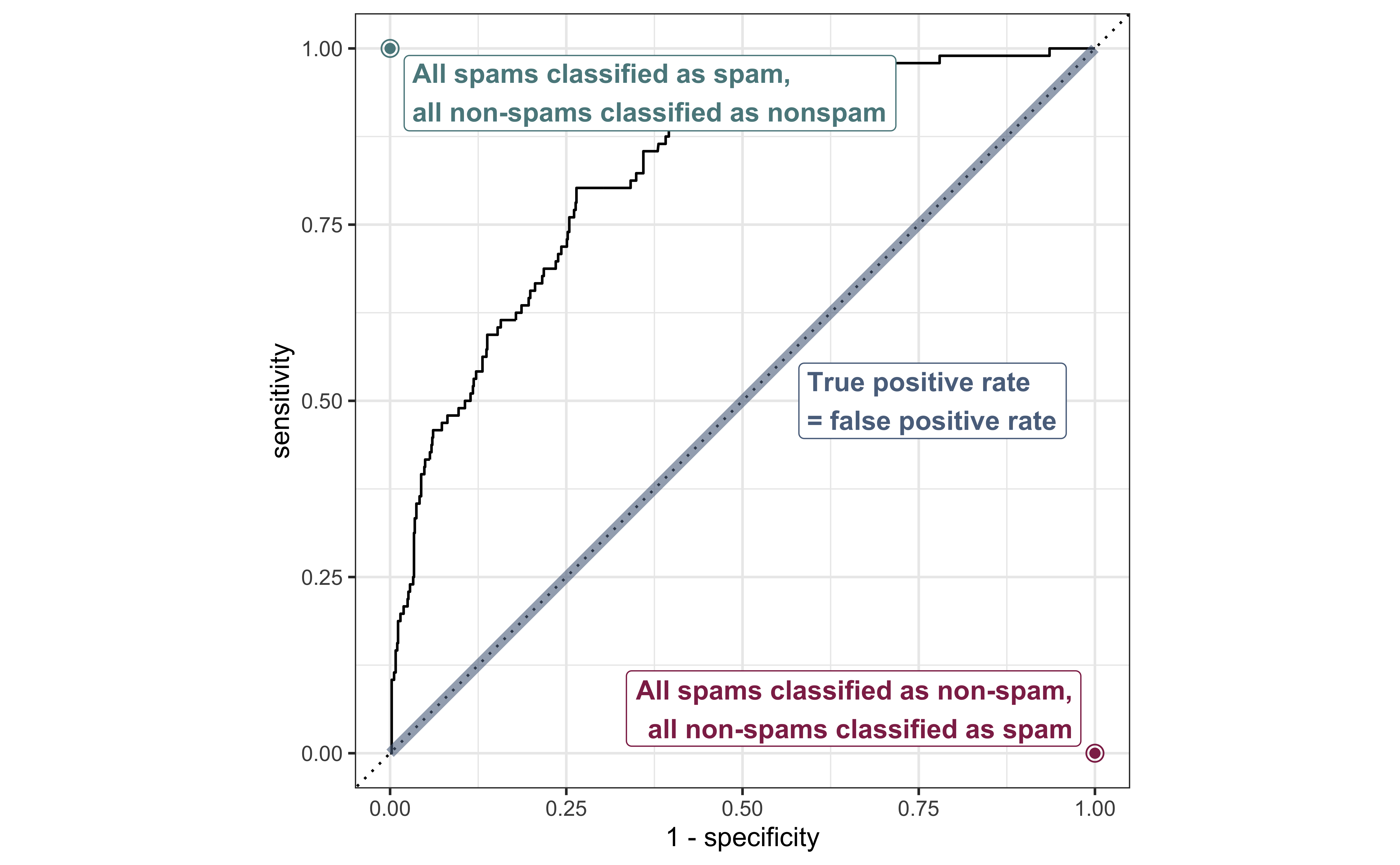
Evaluate the performance: AUC

email_pred |>
  roc_auc(
    truth = spam,
    .pred_1,
    event_level = "second"
  )

# A tibble: 1 × 3
  .metric .estimator .estimate
  <chr>   <chr>          <dbl>
1 roc_auc binary         0.836

The area under the curve (AUC) can be used to assess how well the logistic model fits the data

• AUC=0.5: model is a very bad fit (no better than a coin flip)

• AUC close to 1: model is a good fit

Make decisions

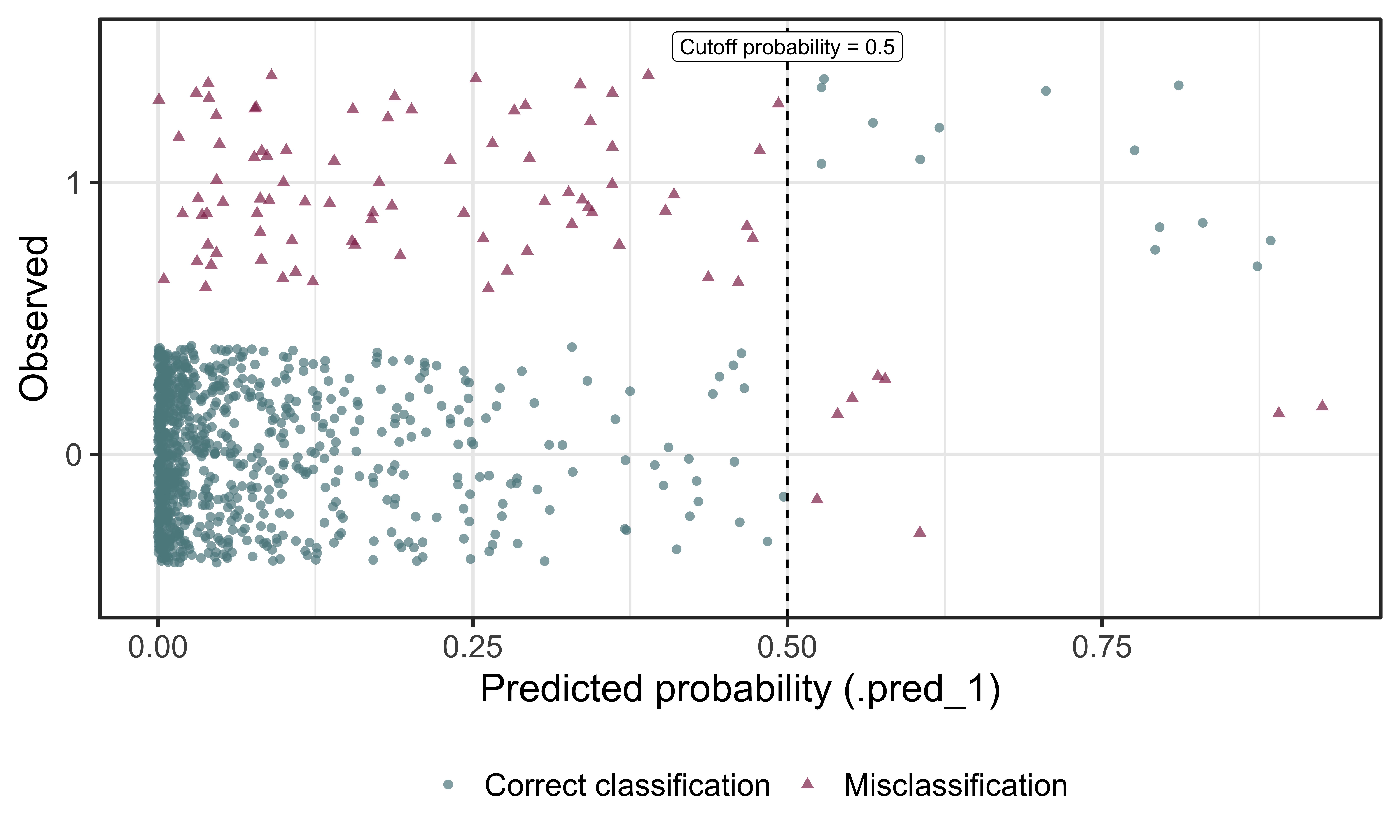
Cutoff probability: 0.5

• Output
• Code

Suppose we decide to label an email as spam if the model predicts the probability of spam to be more than 0.5.

	Email is not spam	Email is spam
Email classified as not spam	877	82
Email classified as spam	8	14

cutoff_prob <- 0.5
email_pred |>
  mutate(
    spam_pred = as_factor(if_else(.pred_1 >= cutoff_prob, 1, 0)),
    spam      = if_else(spam == 1, "Email is spam", "Email is not spam"),
    spam_pred = if_else(spam_pred == 1, "Email classified as spam", "Email classified as not spam")
    ) |>
  count(spam_pred, spam) |>
  pivot_wider(names_from = spam, values_from = n) |>
  kable(col.names = c("", "Email is not spam", "Email is spam"))

Confusion matrix

Cross-tabulation of observed and predicted classes:

cutoff_prob <- 0.5
email_pred |>
  mutate(spam_predicted = as_factor(if_else(.pred_1 >= cutoff_prob, 1, 0))) |>
  conf_mat(truth = spam, estimate = spam_predicted)

          Truth
Prediction   0   1
         0 877  82
         1   8  14

Classification

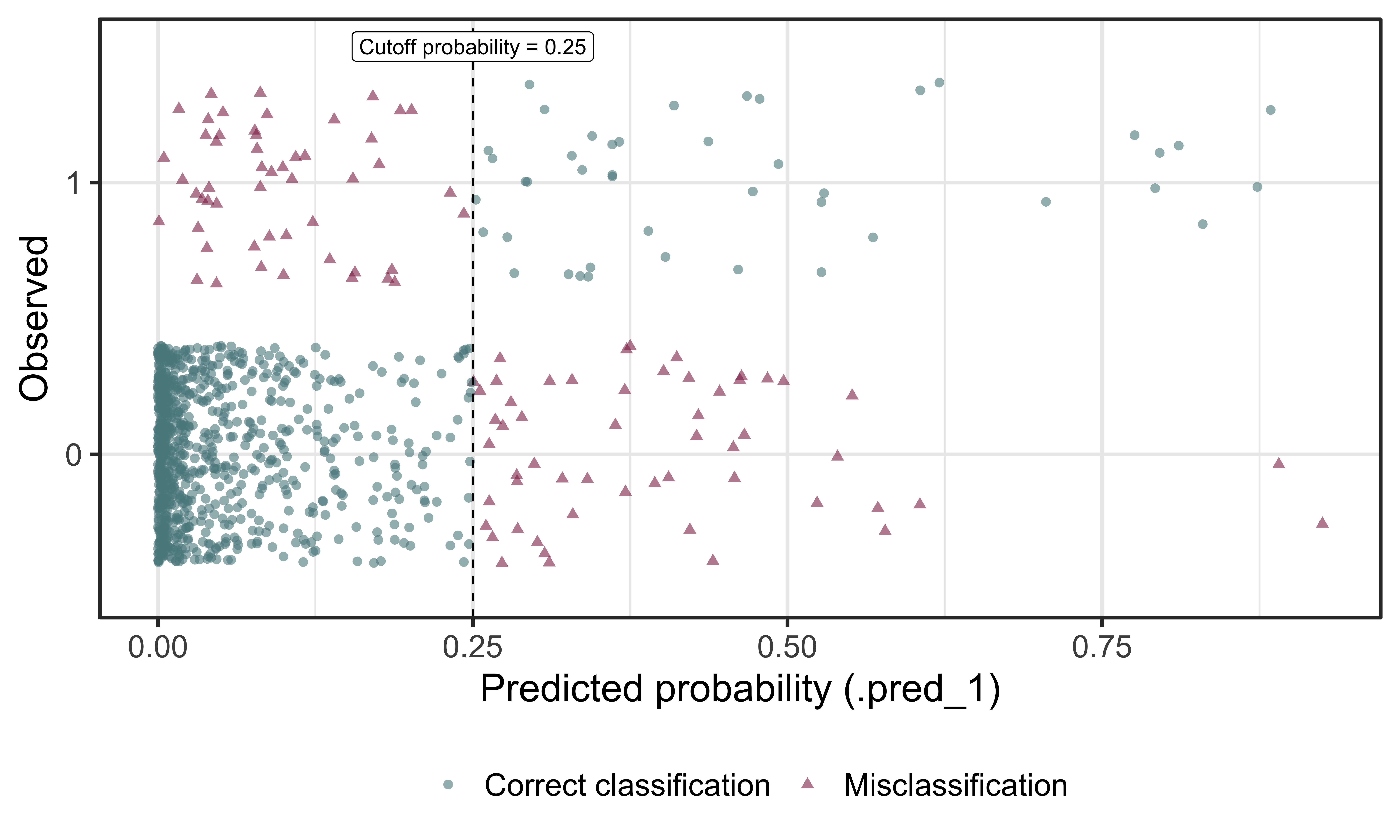
Cutoff probability: 0.25

• Output
• Code

Suppose we decide to label an email as spam if the model predicts the probability of spam to be more than 0.25.

	Email is not spam	Email is spam
Email classified as not spam	830	52
Email classified as spam	55	44

cutoff_prob <- 0.25
email_pred |>
  mutate(
    spam_pred = as_factor(if_else(.pred_1 >= cutoff_prob, 1, 0)),
    spam      = if_else(spam == 1, "Email is spam", "Email is not spam"),
    spam_pred = if_else(spam_pred == 1, "Email classified as spam", "Email classified as not spam")
    ) |>
  count(spam_pred, spam) |>
  pivot_wider(names_from = spam, values_from = n) |>
  kable(col.names = c("", "Email is not spam", "Email is spam"))

Classification

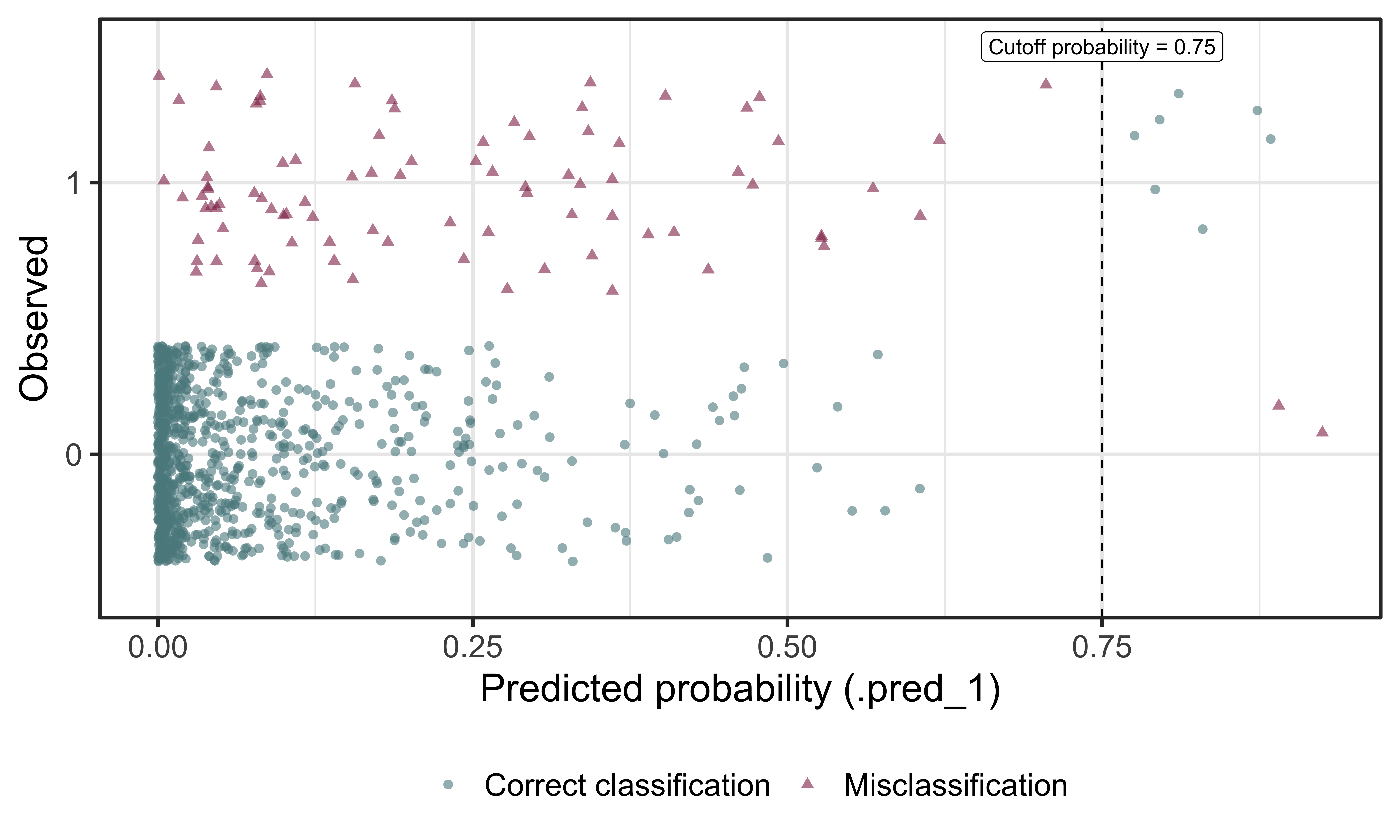
Cutoff probability: 0.75

• Output
• Code

Suppose we decide to label an email as spam if the model predicts the probability of spam to be more than 0.75.

	Email is not spam	Email is spam
Email classified as not spam	883	89
Email classified as spam	2	7

cutoff_prob <- 0.75
email_pred |>
  mutate(
    spam_pred = as_factor(if_else(.pred_1 >= cutoff_prob, 1, 0)),
    spam      = if_else(spam == 1, "Email is spam", "Email is not spam"),
    spam_pred = if_else(spam_pred == 1, "Email classified as spam", "Email classified as not spam")
    ) |>
  count(spam_pred, spam) |>
  pivot_wider(names_from = spam, values_from = n) |>
  kable(col.names = c("", "Email is not spam", "Email is spam"))

Classification

Use ROC curve

Use the ROC curve to determine the best cutoff probability

# A tibble: 10 × 3
   .threshold specificity sensitivity
        <dbl>       <dbl>       <dbl>
 1     0.0769       0.736       0.792
 2     0.0770       0.736       0.781
 3     0.0780       0.737       0.781
 4     0.0785       0.737       0.771
 5     0.0786       0.738       0.771
 6     0.0787       0.739       0.771
 7     0.0789       0.739       0.760
 8     0.0802       0.740       0.760
 9     0.0802       0.741       0.760
10     0.0805       0.742       0.760

Recap

• Built predictive logistic regression models
• Defined and calculated sensitivity and specificity
• Made classification decisions based on sensitivity and specificity