Logistic regression

Introduction

Prof. Maria Tackett

Oct 30, 2023

Announcements

HW 03 due Wed, Nov 1 at 11:59pm
See Ed Discussion for
- Code to reformat Theme variable in HW 03 data set
- Explanation on interpreting models with quadratic terms

Spring 2024 statistics courses

STA 211: Mathematics of Regression
- Prereqs: MATH 216/218/221, STA 210
STA 230 or STA 240: Probability
- Prereqs: MATH 22/112/122/202/212/219/222
STA 310: Generalized Linear Models
- Prereqs: STA 210 and STA 230/240
STA 313: Advanced Data Visualization
- Prereqs: STA 198 or STA 199 or STA 210
STA 323: Statistical Computing
- Prereqs: STA 210 and STA 230/240
STA 360: Bayesian Inference and Modern Statistical Methods
- Prereqs: STA 210 and STA 230/240 and MATH 202/212/219/222 and CS 101/102/201 and MATH 216/218/221, 211 (co-req)

Interpreting models with log-transformed variables

term	estimate	std.error	statistic	p.value
(Intercept)	4.738	0.219	21.667	0.000
hightemp	0.018	0.003	5.452	0.000
seasonSpring	0.026	0.094	0.283	0.778
seasonSummer	-0.047	0.139	-0.338	0.736
cloudcover	-0.025	0.010	-2.452	0.016
precip	-0.294	0.123	-2.397	0.019
day_typeWeekend	0.064	0.065	0.987	0.327

Interpret the intercept in terms of (1) log(volume) and (2) volume.
Interpret the coefficient of hightemp in terms of (1) log(volume) and (2) volume.

Logistic regression

Topics

Logistic regression for binary response variable
Relationship between odds and probabilities
Use logistic regression model to calculate predicted odds and probabilities

Computational setup

# load packages
library(tidyverse)
library(tidymodels)
library(knitr)
library(Stat2Data) #contains data set

# set default theme and larger font size for ggplot2
ggplot2::theme_set(ggplot2::theme_bw(base_size = 20))

Predicting categorical outcomes

Types of outcome variables

Quantitative outcome variable:

Sales price of a house in Duke Forest
Model: Expected sales price given the number of bedrooms, lot size, etc.

Categorical outcome variable:

Indicator of being high risk of getting coronary heart disease in the next 10 years
Model: Probability an adult is high risk of heart disease in the next 10 years given their age, total cholesterol, etc.

Models for categorical outcomes

Logistic regression

2 Outcomes

1: Yes, 0: No

Multinomial logistic regression

3+ Outcomes

1: Democrat, 2: Republican, 3: Independent

2022 election forecasts

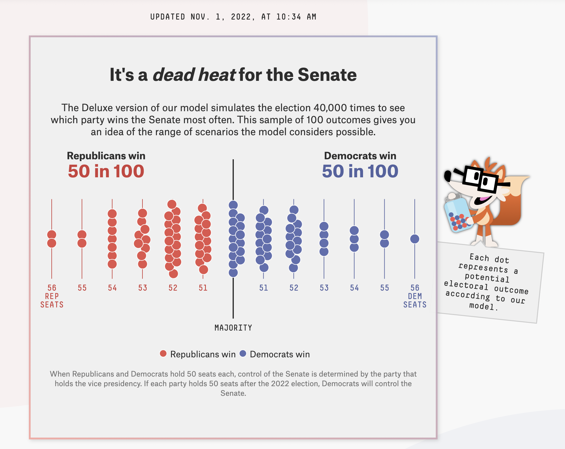
Source: FiveThirtyEight 2022 Election Forecasts

2020 NBA finals predictions

Source: FiveThirtyEight 2019-20 NBA Predictions

Do teenagers get 7+ hours of sleep?

Students in grades 9 - 12 surveyed about health risk behaviors including whether they usually get 7 or more hours of sleep.

Sleep7

1: yes

0: no

data(YouthRisk2009) #from Stat2Data package
sleep <- YouthRisk2009 |>
  as_tibble() |>
  filter(!is.na(Age), !is.na(Sleep7))
sleep |>
  relocate(Age, Sleep7)

# A tibble: 446 × 6
     Age Sleep7 Sleep           SmokeLife SmokeDaily MarijuaEver
   <int>  <int> <fct>           <fct>     <fct>            <int>
 1    16      1 8 hours         Yes       Yes                  1
 2    17      0 5 hours         Yes       Yes                  1
 3    18      0 5 hours         Yes       Yes                  1
 4    17      1 7 hours         Yes       No                   1
 5    15      0 4 or less hours No        No                   0
 6    17      0 6 hours         No        No                   0
 7    17      1 7 hours         No        No                   0
 8    16      1 8 hours         Yes       No                   0
 9    16      1 8 hours         No        No                   0
10    18      0 4 or less hours Yes       Yes                  1
# ℹ 436 more rows

Plot the data

ggplot(sleep, aes(x = Age, y = Sleep7)) +
  geom_point() + 
  labs(y = "Getting 7+ hours of sleep")

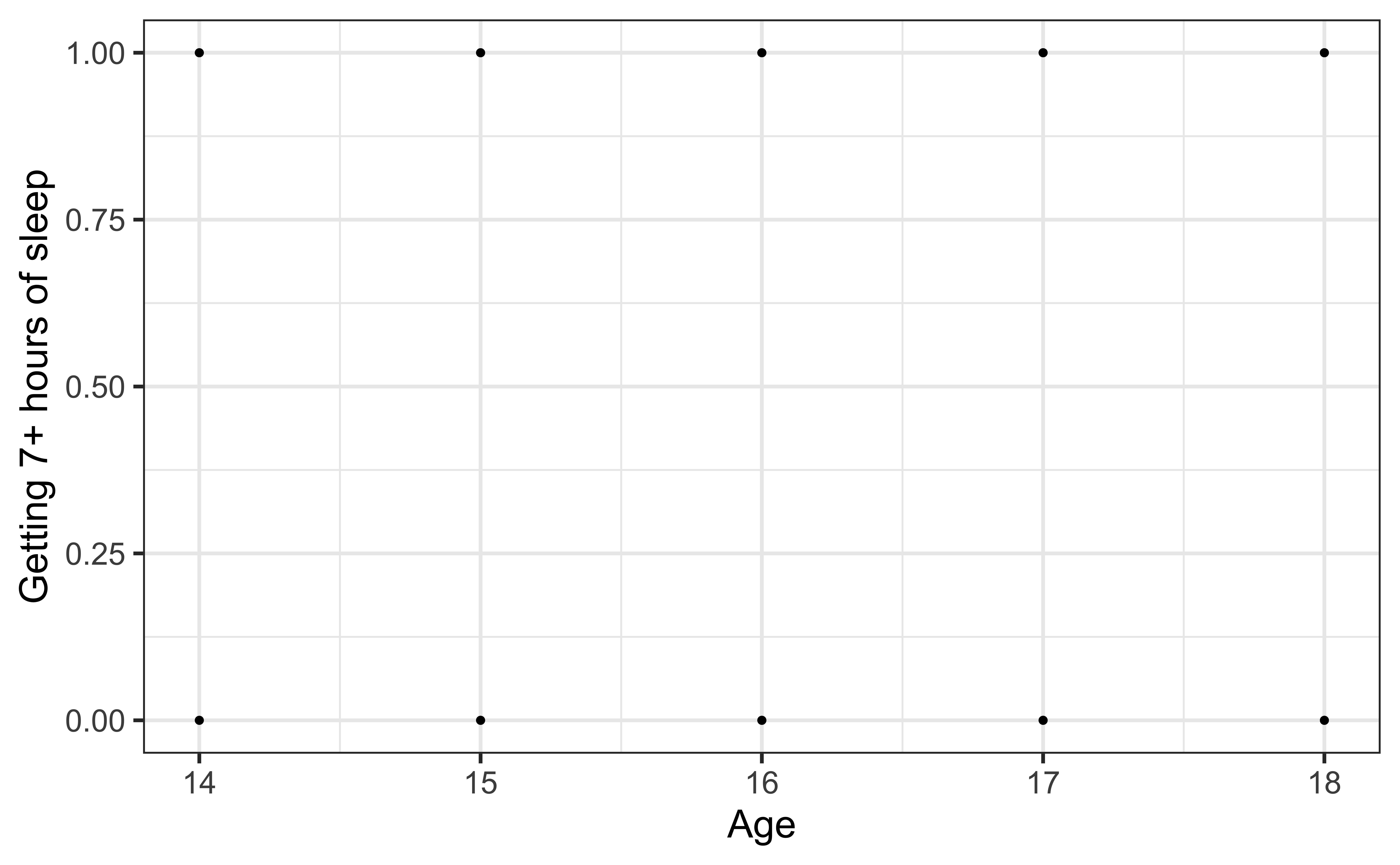
Let’s fit a linear regression model

Outcome: \(Y\) = 1: yes, 0: no

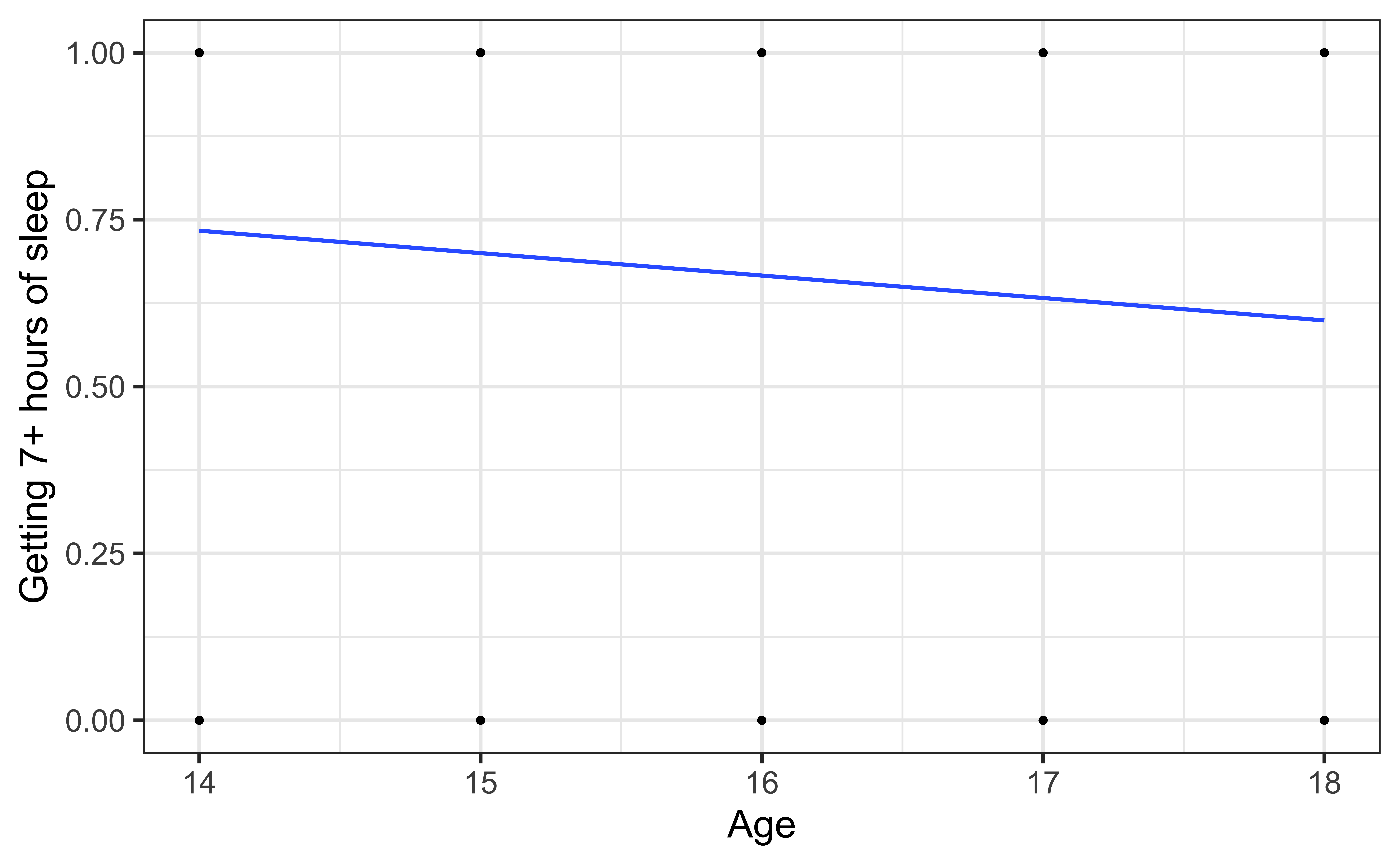
Let’s use proportions

Outcome: Probability of getting 7+ hours of sleep

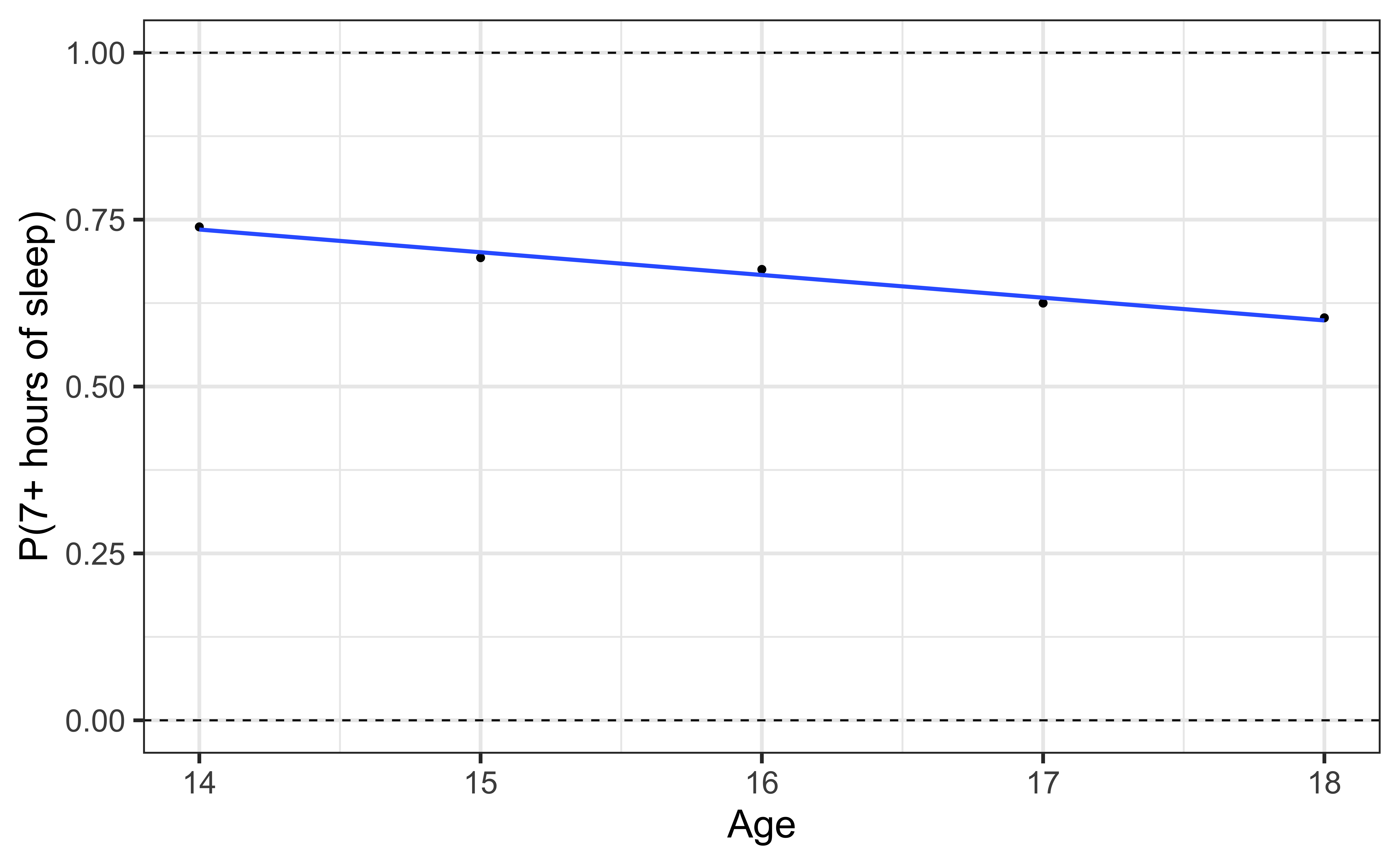
What happens if we zoom out?

Outcome: Probability of getting 7+ hours of sleep

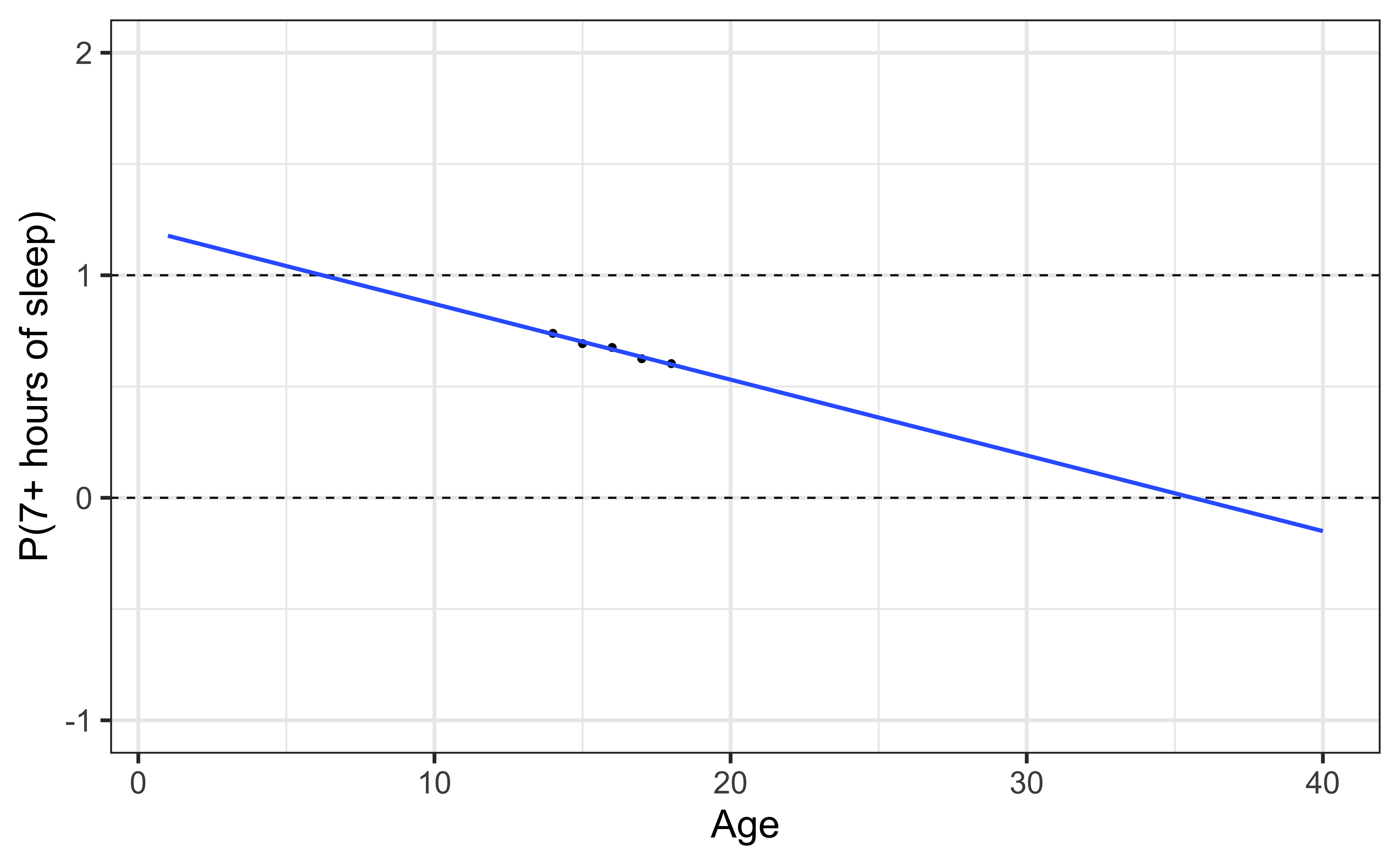
🛑 This model produces predictions outside of 0 and 1.

Let’s try another model

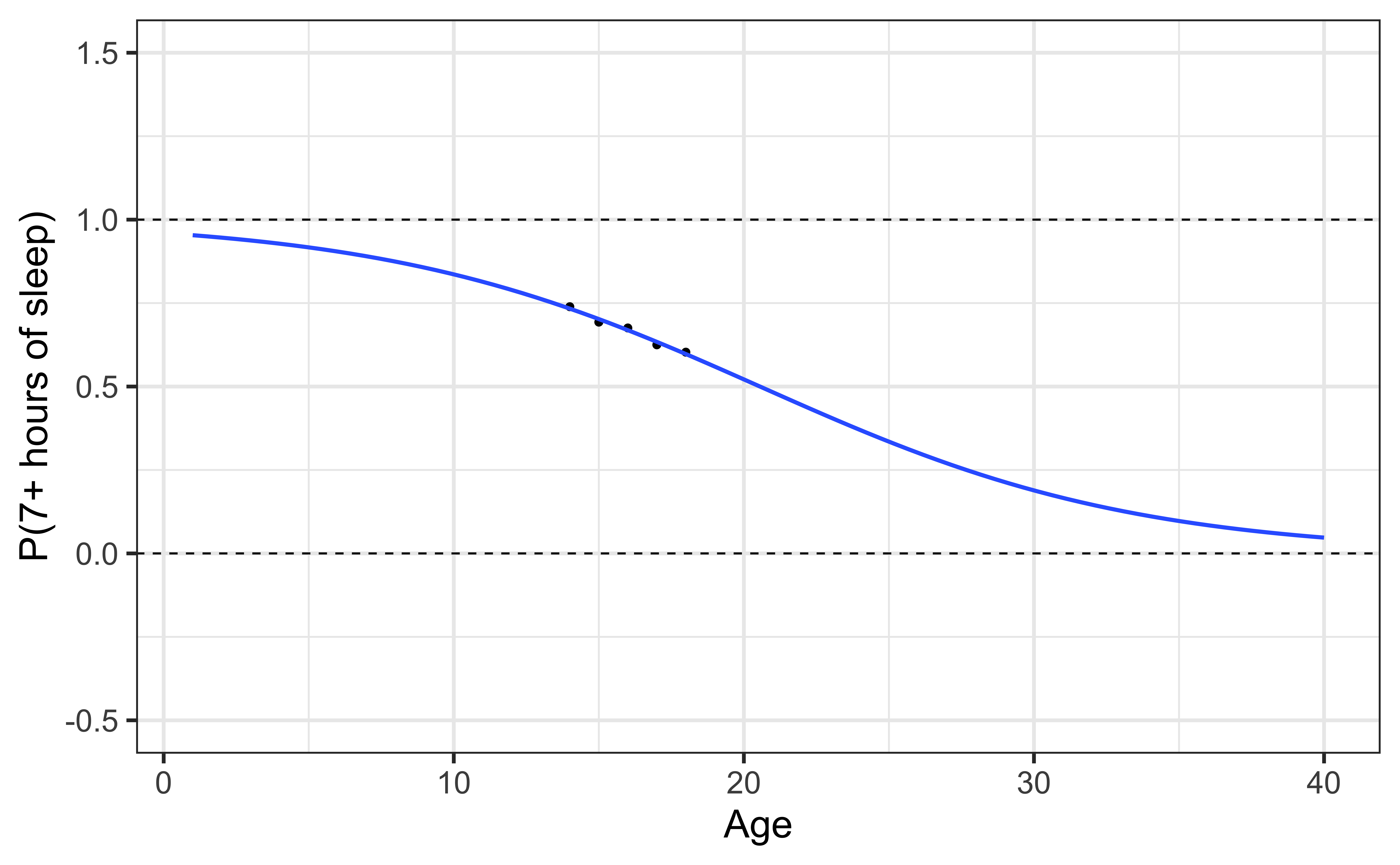
✅ This model (called a logistic regression model) only produces predictions between 0 and 1.

The code

ggplot(sleep_age, aes(x = Age, y = prop)) +
  geom_point() + 
  geom_hline(yintercept = c(0,1), lty = 2) + 
  stat_smooth(method ="glm", method.args = list(family = "binomial"), 
              fullrange = TRUE, se = FALSE) +
  labs(y = "P(7+ hours of sleep)") +
  xlim(1, 40) +
  ylim(-0.5, 1.5)

Different types of models

Method	Outcome	Model
Linear regression	Quantitative	\(Y = \beta_0 + \beta_1~ X\)
Linear regression (transform Y)	Quantitative	\(\log(Y) = \beta_0 + \beta_1~ X\)
Logistic regression	Binary	\(\log\big(\frac{\pi}{1-\pi}\big) = \beta_0 + \beta_1 ~ X\)

Linear vs. logistic regression

State whether a linear regression model or logistic regression model is more appropriate for each scenario.

Use age and education to predict if a randomly selected person will vote in the next election.
Use budget and run time (in minutes) to predict a movie’s total revenue.
Use age and sex to calculate the probability a randomly selected adult will visit Duke Health in the next year.

Submit your responses on Ed Discussion [10:05am][1:25pm]

Odds and probabilities

Binary response variable

\(Y = 1: \text{ yes}, 0: \text{ no}\)
\(\pi\): probability that \(Y=1\), i.e., \(P(Y = 1)\)
\(\frac{\pi}{1-\pi}\): odds that \(Y = 1\)
\(\log\big(\frac{\pi}{1-\pi}\big)\): log odds
Go from \(\pi\) to \(\log\big(\frac{\pi}{1-\pi}\big)\) using the logit transformation

Odds

Suppose there is a 70% chance it will rain tomorrow

Probability it will rain is \(\mathbf{p = 0.7}\)
Probability it won’t rain is \(\mathbf{1 - p = 0.3}\)
Odds it will rain are 7 to 3, 7:3, \(\mathbf{\frac{0.7}{0.3} \approx 2.33}\)

Are teenagers getting enough sleep?

sleep |>
  count(Sleep7) |>
  mutate(p = round(n / sum(n), 3))

# A tibble: 2 × 3
  Sleep7     n     p
   <int> <int> <dbl>
1      0   150 0.336
2      1   296 0.664

\(P(\text{7+ hours of sleep}) = P(Y = 1) = p = 0.664\)

\(P(\text{< 7 hours of sleep}) = P(Y = 0) = 1 - p = 0.336\)

\(P(\text{odds of 7+ hours of sleep}) = \frac{0.664}{0.336} = 1.976\)

From odds to probabilities

odds

\[\omega = \frac{\pi}{1-\pi}\]

probability

\[\pi = \frac{\omega}{1 + \omega}\]

Logistic regression

From odds to probabilities

Logistic model: log odds = \(\log\big(\frac{\pi}{1-\pi}\big) = \beta_0 + \beta_1~X\)
Odds = \(\exp\big\{\log\big(\frac{\pi}{1-\pi}\big)\big\} = \frac{\pi}{1-\pi}\)
Combining (1) and (2) with what we saw earlier

\[\text{probability} = \pi = \frac{\exp\{\beta_0 + \beta_1~X\}}{1 + \exp\{\beta_0 + \beta_1~X\}}\]

Logistic regression model

Logit form: \[\log\big(\frac{\pi}{1-\pi}\big) = \beta_0 + \beta_1~X\]

Probability form:

\[ \pi = \frac{\exp\{\beta_0 + \beta_1~X\}}{1 + \exp\{\beta_0 + \beta_1~X\}} \]

Risk of coronary heart disease

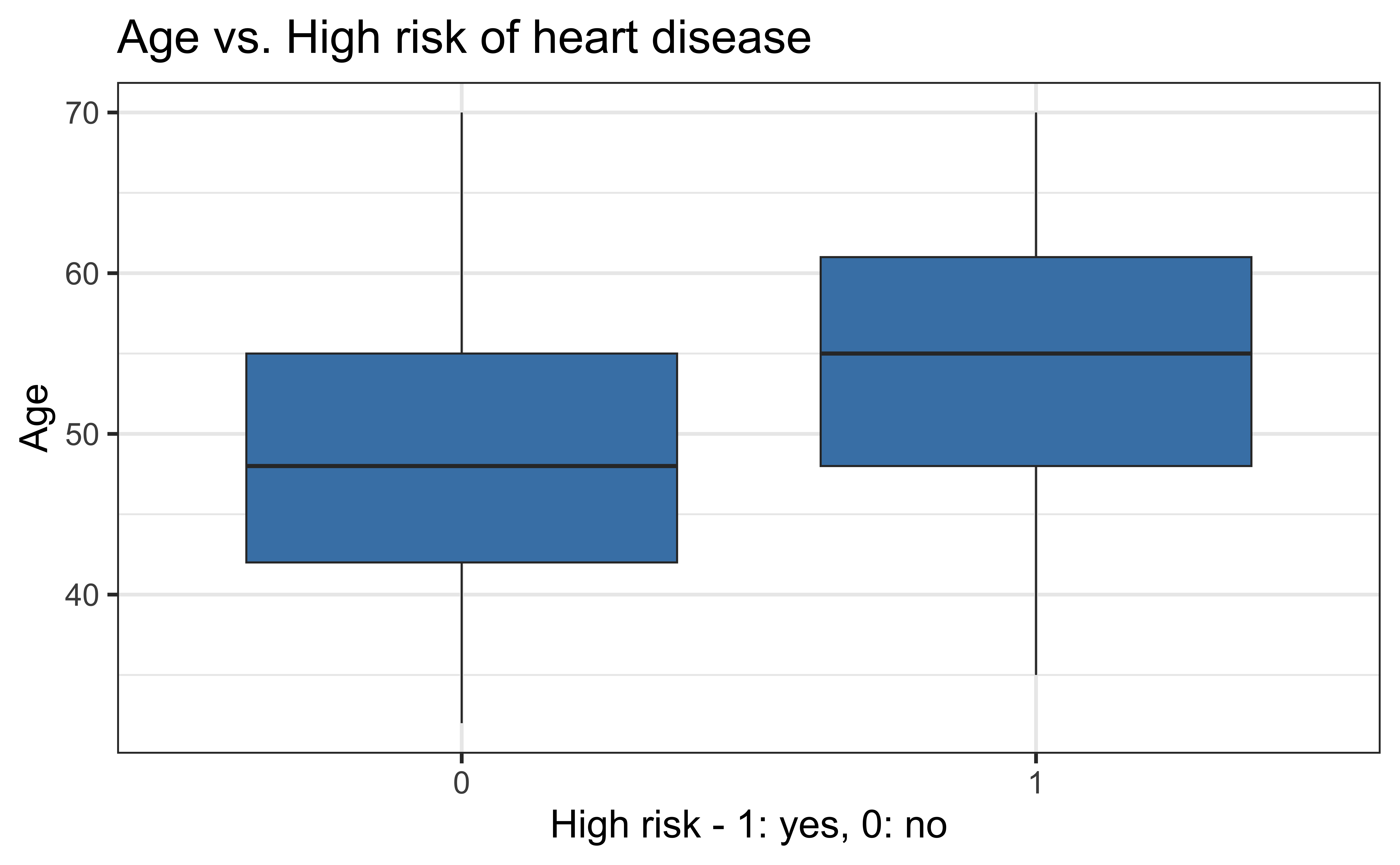
This dataset is from an ongoing cardiovascular study on residents of the town of Framingham, Massachusetts. We want to use age to predict if a randomly selected adult is high risk of having coronary heart disease in the next 10 years.

high_risk:

1: High risk of having heart disease in next 10 years
0: Not high risk of having heart disease in next 10 years

age: Age at exam time (in years)

Data: `heart_disease`

# A tibble: 4,240 × 2
     age high_risk
   <dbl> <fct>    
 1    39 0        
 2    46 0        
 3    48 0        
 4    61 1        
 5    46 0        
 6    43 0        
 7    63 1        
 8    45 0        
 9    52 0        
10    43 0        
# ℹ 4,230 more rows

High risk vs. age

ggplot(heart_disease, aes(x = high_risk, y = age)) +
  geom_boxplot(fill = "steelblue") +
  labs(x = "High risk - 1: yes, 0: no",
       y = "Age", 
       title = "Age vs. High risk of heart disease")

Let’s fit the model

heart_disease_fit <- logistic_reg() |>
  set_engine("glm") |>
  fit(high_risk ~ age, data = heart_disease, family = "binomial")

tidy(heart_disease_fit) |> kable(digits = 3)

term	estimate	std.error	statistic	p.value
(Intercept)	-5.561	0.284	-19.599	0
age	0.075	0.005	14.178	0

The model

tidy(heart_disease_fit) |> kable(digits = 3)

term	estimate	std.error	statistic	p.value
(Intercept)	-5.561	0.284	-19.599	0
age	0.075	0.005	14.178	0

\[\log\Big(\frac{\hat{\pi}}{1-\hat{\pi}}\Big) = -5.561 + 0.075 \times \text{age}\] where \(\hat{\pi}\) is the predicted probability of being high risk of having heart disease in the next 10 years

Predicted log odds

augment(heart_disease_fit$fit) |> select(.fitted, .resid)

# A tibble: 4,240 × 2
   .fitted .resid
     <dbl>  <dbl>
 1  -2.65  -0.370
 2  -2.13  -0.475
 3  -1.98  -0.509
 4  -1.01   1.62 
 5  -2.13  -0.475
 6  -2.35  -0.427
 7  -0.858  1.56 
 8  -2.20  -0.458
 9  -1.68  -0.585
10  -2.35  -0.427
# ℹ 4,230 more rows

For observation 1

\[\text{predicted odds} = \hat{\omega} = \frac{\hat{\pi}}{1-\hat{\pi}} = \exp\{-2.650\} = 0.071\]

Predicted probabilities

predict(heart_disease_fit, new_data = heart_disease, type = "prob")

# A tibble: 4,240 × 2
   .pred_0 .pred_1
     <dbl>   <dbl>
 1   0.934  0.0660
 2   0.894  0.106 
 3   0.878  0.122 
 4   0.733  0.267 
 5   0.894  0.106 
 6   0.913  0.0870
 7   0.702  0.298 
 8   0.900  0.0996
 9   0.843  0.157 
10   0.913  0.0870
# ℹ 4,230 more rows

For observation 1

\[\text{predicted probability} = \hat{\pi} = \frac{\exp\{-2.650\}}{1 + \exp\{-2.650\}} = 0.066\]

Predicted classes

predict(heart_disease_fit, new_data = heart_disease, type = "class")

# A tibble: 4,240 × 1
   .pred_class
   <fct>      
 1 0          
 2 0          
 3 0          
 4 0          
 5 0          
 6 0          
 7 0          
 8 0          
 9 0          
10 0          
# ℹ 4,230 more rows

Default prediction

For a logistic regression, the default prediction is the class.

predict(heart_disease_fit, new_data = heart_disease)

# A tibble: 4,240 × 1
   .pred_class
   <fct>      
 1 0          
 2 0          
 3 0          
 4 0          
 5 0          
 6 0          
 7 0          
 8 0          
 9 0          
10 0          
# ℹ 4,230 more rows

Observed vs. predicted

What does the following table show?

predict(heart_disease_fit, new_data = heart_disease) |>
  bind_cols(heart_disease) |>
  count(high_risk, .pred_class)

# A tibble: 2 × 3
  high_risk .pred_class     n
  <fct>     <fct>       <int>
1 0         0            3596
2 1         0             644

The .pred_class is the class with the highest predicted probability. What is a limitation to using this method to determine the predicted class?

Application exercise

📋 AE 12: Logistic Regression Intro

Recap

Introduced logistic regression for binary response variable
Described relationship between odds and probabilities
Used logistic regression model to calculate predicted odds and probabilities

Logistic regression

Announcements

Spring 2024 statistics courses

Interpreting models with log-transformed variables

Logistic regression

Topics

Computational setup

Predicting categorical outcomes

Types of outcome variables

Models for categorical outcomes

2022 election forecasts

2020 NBA finals predictions

Do teenagers get 7+ hours of sleep?

Plot the data

Let’s fit a linear regression model

Let’s use proportions

What happens if we zoom out?

Let’s try another model

The code

Different types of models

Linear vs. logistic regression

Odds and probabilities

Binary response variable

Odds

Are teenagers getting enough sleep?

From odds to probabilities

Logistic regression

From odds to probabilities

Logistic regression model

Risk of coronary heart disease

Data: heart_disease

High risk vs. age

Let’s fit the model

The model

Predicted log odds

Predicted probabilities

Predicted classes

Default prediction

Observed vs. predicted

Application exercise

Recap

Data: `heart_disease`