Simple Linear Regression

Prof. Maria Tackett

Sep 06, 2023

Questions?

Join sta210-fa23 on GitHub

Topics

Use simple linear regression to describe the relationship between a quantitative predictor and quantitative response variable.
Estimate the slope and intercept of the regression line using the least squares method.
Interpret the slope and intercept of the regression line.
Predict the response given a value of the predictor variable.
Use tidymodels to fit and summarize regression models in R.

Computation set up

# load packages
library(tidyverse)       # for data wrangling
library(tidymodels)      # for modeling
library(fivethirtyeight) # for the fandango dataset
library(knitr)          # for formatting tables

# set default theme and larger font size for ggplot2
ggplot2::theme_set(ggplot2::theme_bw(base_size = 16))

# set default figure parameters for knitr
knitr::opts_chunk$set(
  fig.width = 8,
  fig.asp = 0.618,
  fig.retina = 3,
  dpi = 300,
  out.width = "80%"
)

Data

Movie scores

Data behind the FiveThirtyEight story Be Suspicious Of Online Movie Ratings, Especially Fandango’s
In the fivethirtyeight package: fandango
Contains every film released in 2014 and 2015 that has at least 30 fan reviews on Fandango, an IMDb score, Rotten Tomatoes critic and user ratings, and Metacritic critic and user scores

Fandango logo

IMDB logo

Rotten Tomatoes logo

Metacritic logo

Data prep

Rename Rotten Tomatoes columns as critics and audience
Rename the dataset as movie_scores

movie_scores <- fandango |>
  rename(critics = rottentomatoes, 
         audience = rottentomatoes_user)

Data overview

glimpse(movie_scores)

Rows: 146
Columns: 23
$ film                       <chr> "Avengers: Age of Ultron", "Cinderella", "A…
$ year                       <dbl> 2015, 2015, 2015, 2015, 2015, 2015, 2015, 2…
$ critics                    <int> 74, 85, 80, 18, 14, 63, 42, 86, 99, 89, 84,…
$ audience                   <int> 86, 80, 90, 84, 28, 62, 53, 64, 82, 87, 77,…
$ metacritic                 <int> 66, 67, 64, 22, 29, 50, 53, 81, 81, 80, 71,…
$ metacritic_user            <dbl> 7.1, 7.5, 8.1, 4.7, 3.4, 6.8, 7.6, 6.8, 8.8…
$ imdb                       <dbl> 7.8, 7.1, 7.8, 5.4, 5.1, 7.2, 6.9, 6.5, 7.4…
$ fandango_stars             <dbl> 5.0, 5.0, 5.0, 5.0, 3.5, 4.5, 4.0, 4.0, 4.5…
$ fandango_ratingvalue       <dbl> 4.5, 4.5, 4.5, 4.5, 3.0, 4.0, 3.5, 3.5, 4.0…
$ rt_norm                    <dbl> 3.70, 4.25, 4.00, 0.90, 0.70, 3.15, 2.10, 4…
$ rt_user_norm               <dbl> 4.30, 4.00, 4.50, 4.20, 1.40, 3.10, 2.65, 3…
$ metacritic_norm            <dbl> 3.30, 3.35, 3.20, 1.10, 1.45, 2.50, 2.65, 4…
$ metacritic_user_nom        <dbl> 3.55, 3.75, 4.05, 2.35, 1.70, 3.40, 3.80, 3…
$ imdb_norm                  <dbl> 3.90, 3.55, 3.90, 2.70, 2.55, 3.60, 3.45, 3…
$ rt_norm_round              <dbl> 3.5, 4.5, 4.0, 1.0, 0.5, 3.0, 2.0, 4.5, 5.0…
$ rt_user_norm_round         <dbl> 4.5, 4.0, 4.5, 4.0, 1.5, 3.0, 2.5, 3.0, 4.0…
$ metacritic_norm_round      <dbl> 3.5, 3.5, 3.0, 1.0, 1.5, 2.5, 2.5, 4.0, 4.0…
$ metacritic_user_norm_round <dbl> 3.5, 4.0, 4.0, 2.5, 1.5, 3.5, 4.0, 3.5, 4.5…
$ imdb_norm_round            <dbl> 4.0, 3.5, 4.0, 2.5, 2.5, 3.5, 3.5, 3.5, 3.5…
$ metacritic_user_vote_count <int> 1330, 249, 627, 31, 88, 34, 17, 124, 62, 54…
$ imdb_user_vote_count       <int> 271107, 65709, 103660, 3136, 19560, 39373, …
$ fandango_votes             <int> 14846, 12640, 12055, 1793, 1021, 397, 252, …
$ fandango_difference        <dbl> 0.5, 0.5, 0.5, 0.5, 0.5, 0.5, 0.5, 0.5, 0.5…

Movie scores data

The data set contains the “Tomatometer” score (critics) and audience score (audience) for 146 movies rated on rottentomatoes.com.

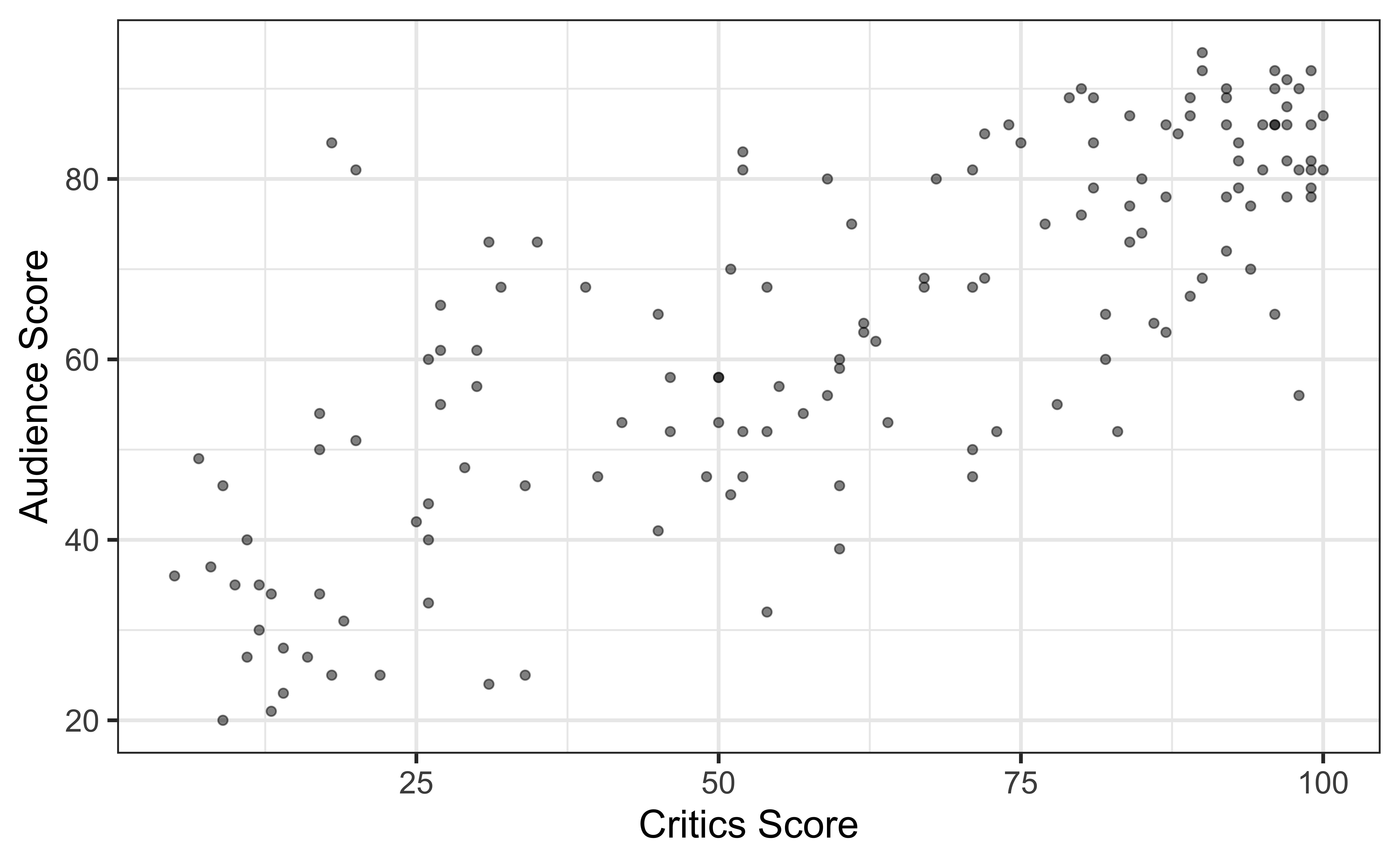
Movie ratings data

Goal: Fit a line to describe the relationship between the critics score and audience score.

`geom_smooth()` using formula = 'y ~ x'

Why fit a line?

We fit a line to accomplish one or both of the following:

Prediction

What is the audience score expected to be for an upcoming movie that received 35% from the critics?

Inference

Is the critics score a useful predictor of the audience score? By how much is the audience score expected to change for each additional point in the critics score?

Terminology

Response, Y: variable describing the outcome of interest
Predictor, X: variable we use to help understand the variability in the response

`geom_smooth()` using formula = 'y ~ x'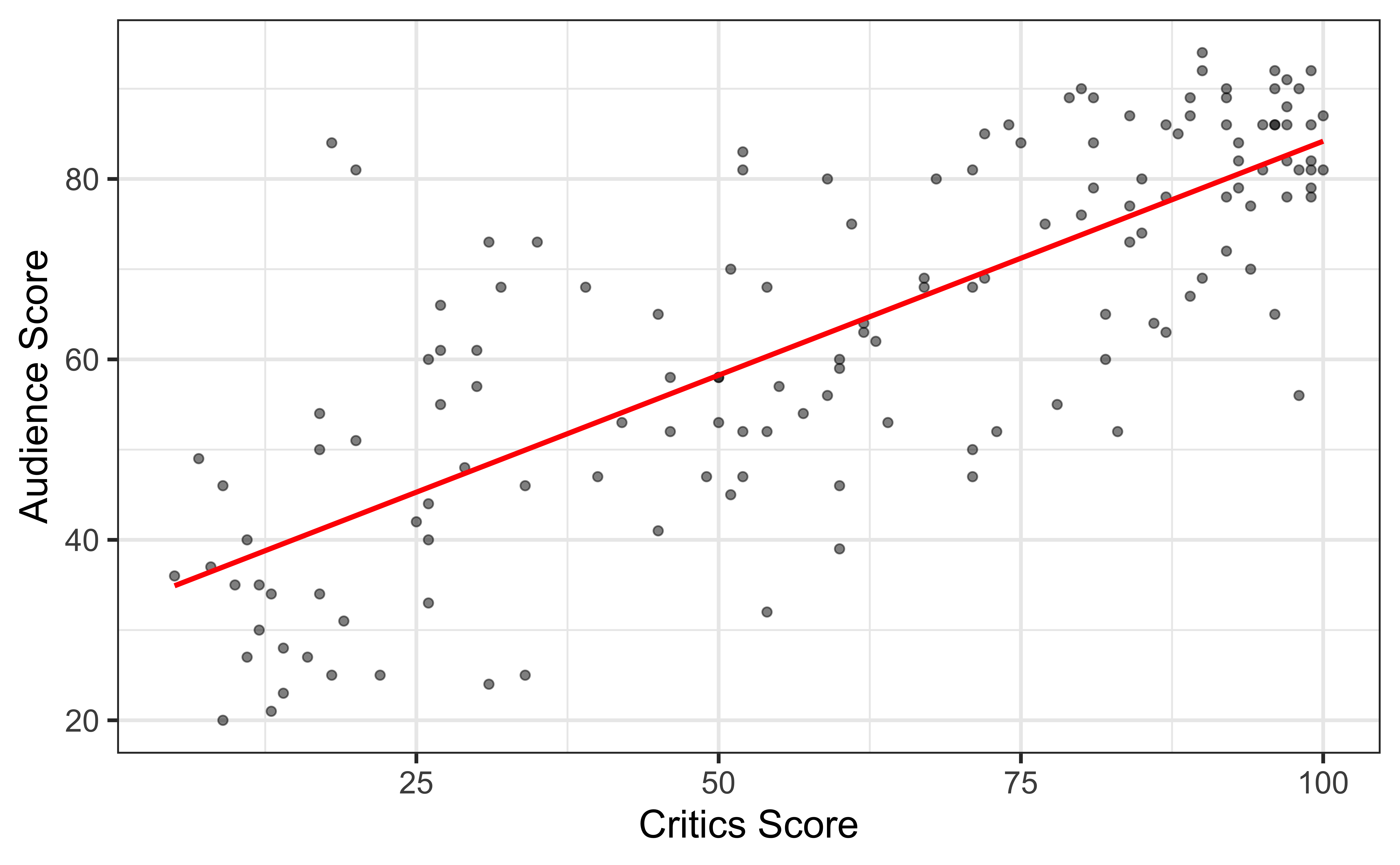

Regression model

A regression model is a function that describes the relationship between the response, \(Y\), and the predictor, \(X\).

\[\begin{aligned} Y &= \color{black}{\textbf{Model}} + \text{Error} \\[8pt] &= \color{black}{\mathbf{f(X)}} + \epsilon \\[8pt] &= \color{black}{\boldsymbol{\mu_{Y|X}}} + \epsilon \end{aligned}\]

Regression model

\[\begin{aligned} Y &= \color{purple}{\textbf{Model}} + \text{Error} \\[8pt] &= \color{purple}{\mathbf{f(X)}} + \epsilon \\[8pt] &= \color{purple}{\boldsymbol{\mu_{Y|X}}} + \epsilon \end{aligned}\]

`geom_smooth()` using formula = 'y ~ x'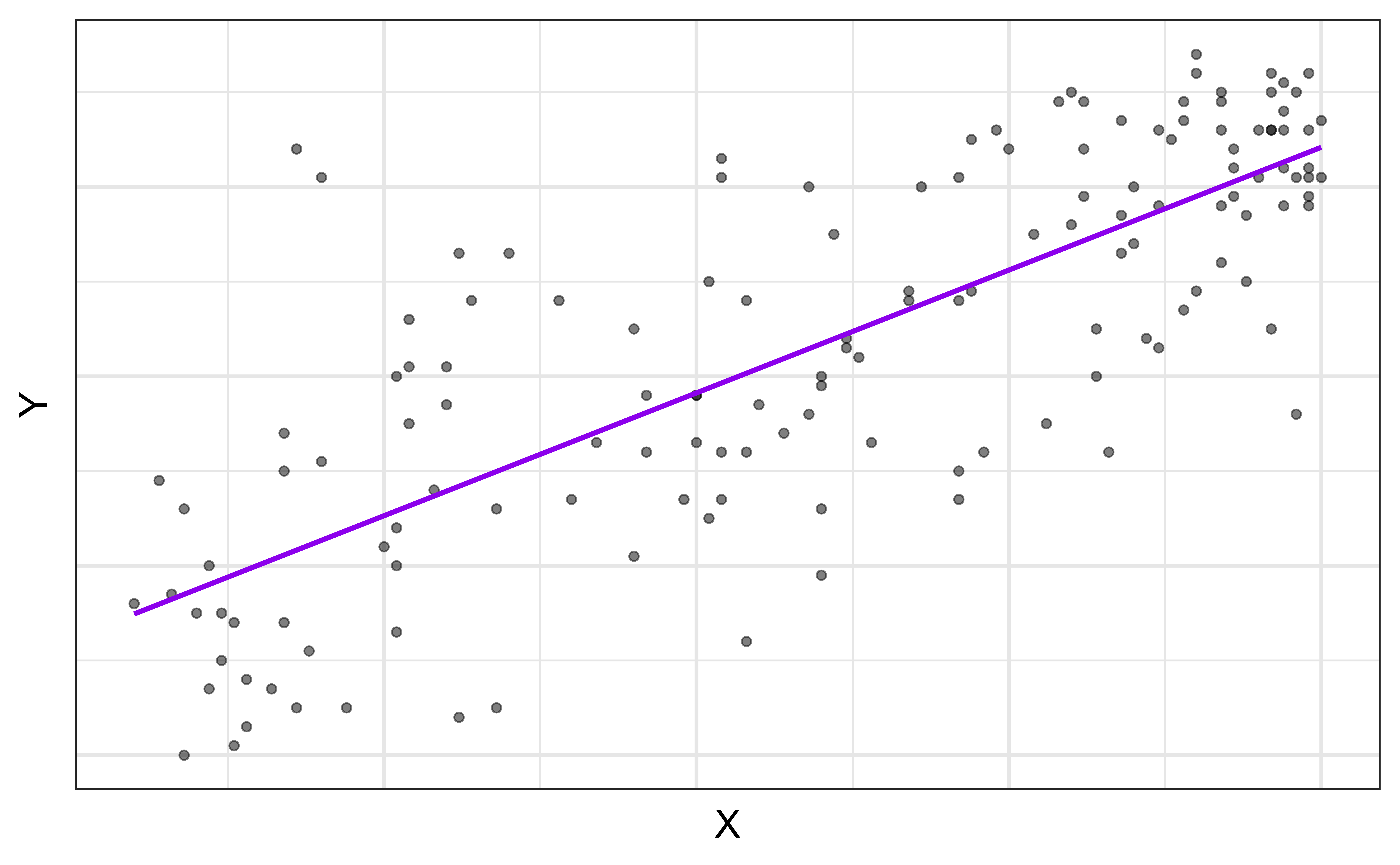

\(\mu_{Y|X}\) is the mean value of \(Y\) given a particular value of \(X\).

Regression model

\[ \begin{aligned} Y &= \color{purple}{\textbf{Model}} + \color{blue}{\textbf{Error}} \\[5pt] &= \color{purple}{\mathbf{f(X)}} + \color{blue}{\boldsymbol{\epsilon}} \\[5pt] &= \color{purple}{\boldsymbol{\mu_{Y|X}}} + \color{blue}{\boldsymbol{\epsilon}} \\[5pt] \end{aligned} \]

`geom_smooth()` using formula = 'y ~ x'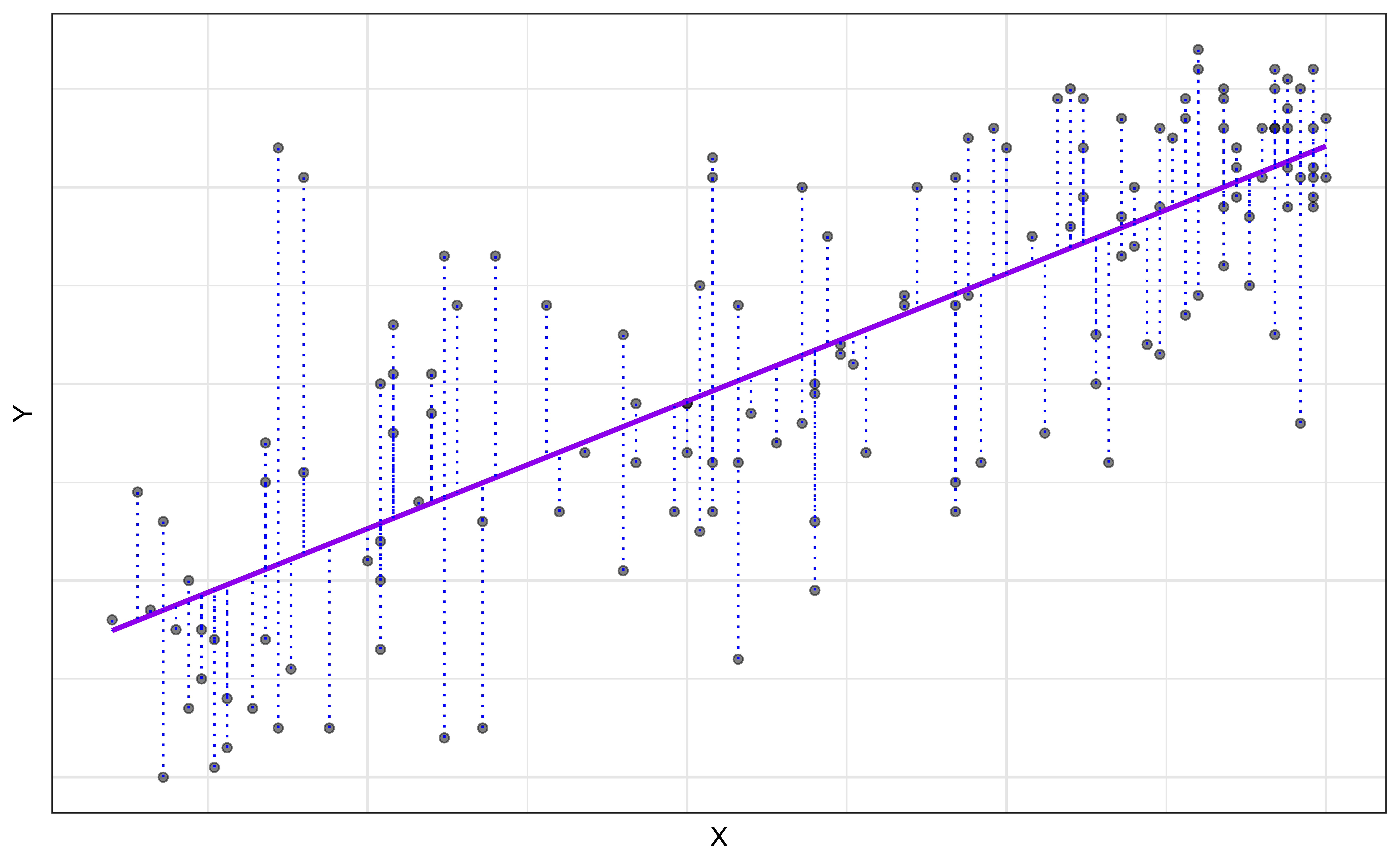

Simple linear regression (SLR)

SLR: Statistical model

When we have a quantitative response, \(Y\), and a single quantitative predictor, \(X\), we can use a simple linear regression model to describe the relationship between \(Y\) and \(X\). \[\Large{Y = \mathbf{\beta_0 + \beta_1 X} + \epsilon}\]

\(\beta_1\): True slope of the relationship between \(X\) and \(Y\)
\(\beta_0\): True intercept of the relationship between \(X\) and \(Y\)
\(\epsilon\): Error

SLR: Regression equation

\[\Large{\hat{Y} = \hat{\beta}_0 + \hat{\beta}_1 X}\]

\(\hat{\beta}_1\): Estimated slope of the relationship between \(X\) and \(Y\)
\(\hat{\beta}_0\): Estimated intercept of the relationship between \(X\) and \(Y\)
No error term!

Choosing values for \(\hat{\beta}_1\) and \(\hat{\beta}_0\)

Warning: Using `size` aesthetic for lines was deprecated in ggplot2 3.4.0.
ℹ Please use `linewidth` instead.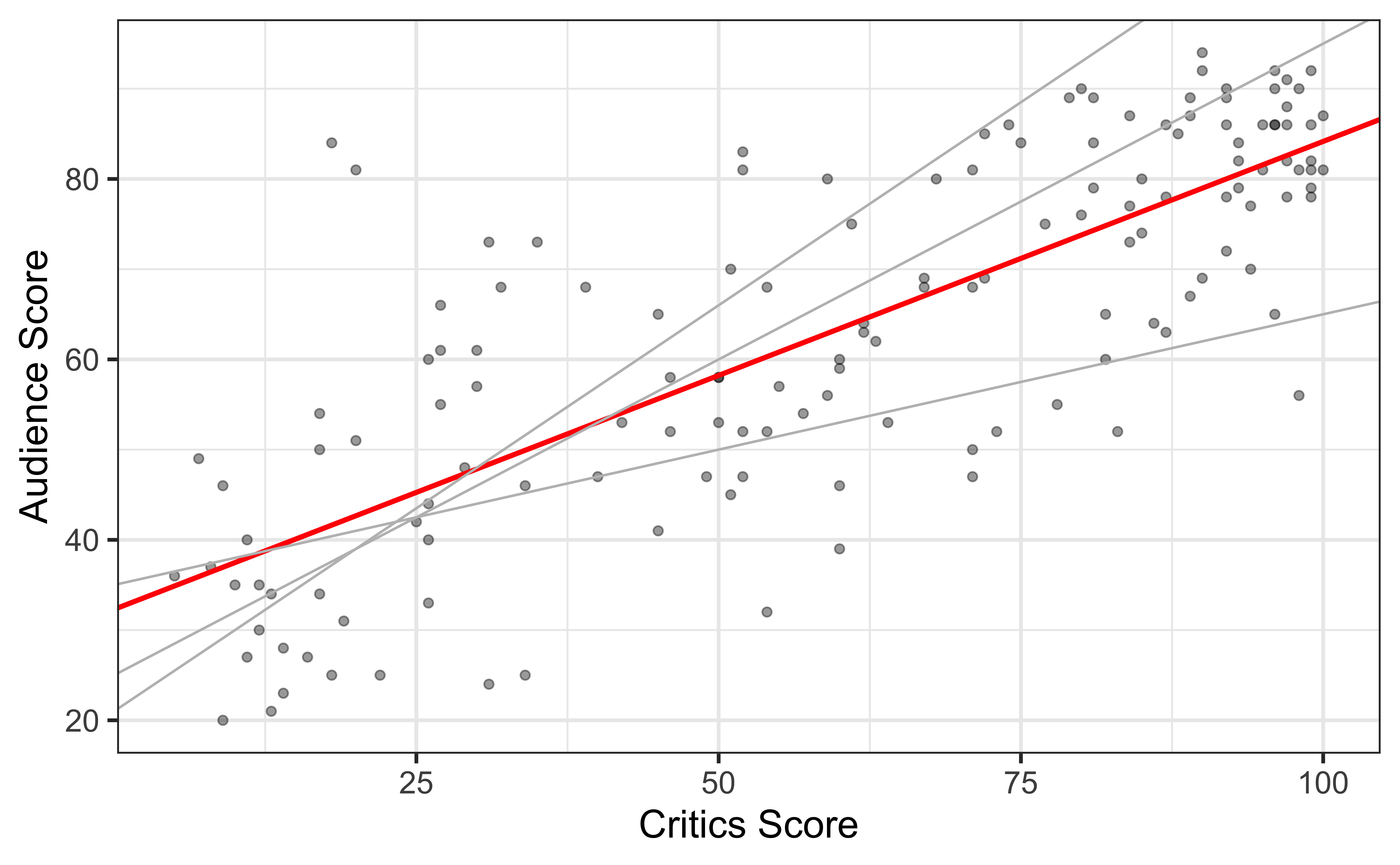

Residuals

`geom_smooth()` using formula = 'y ~ x'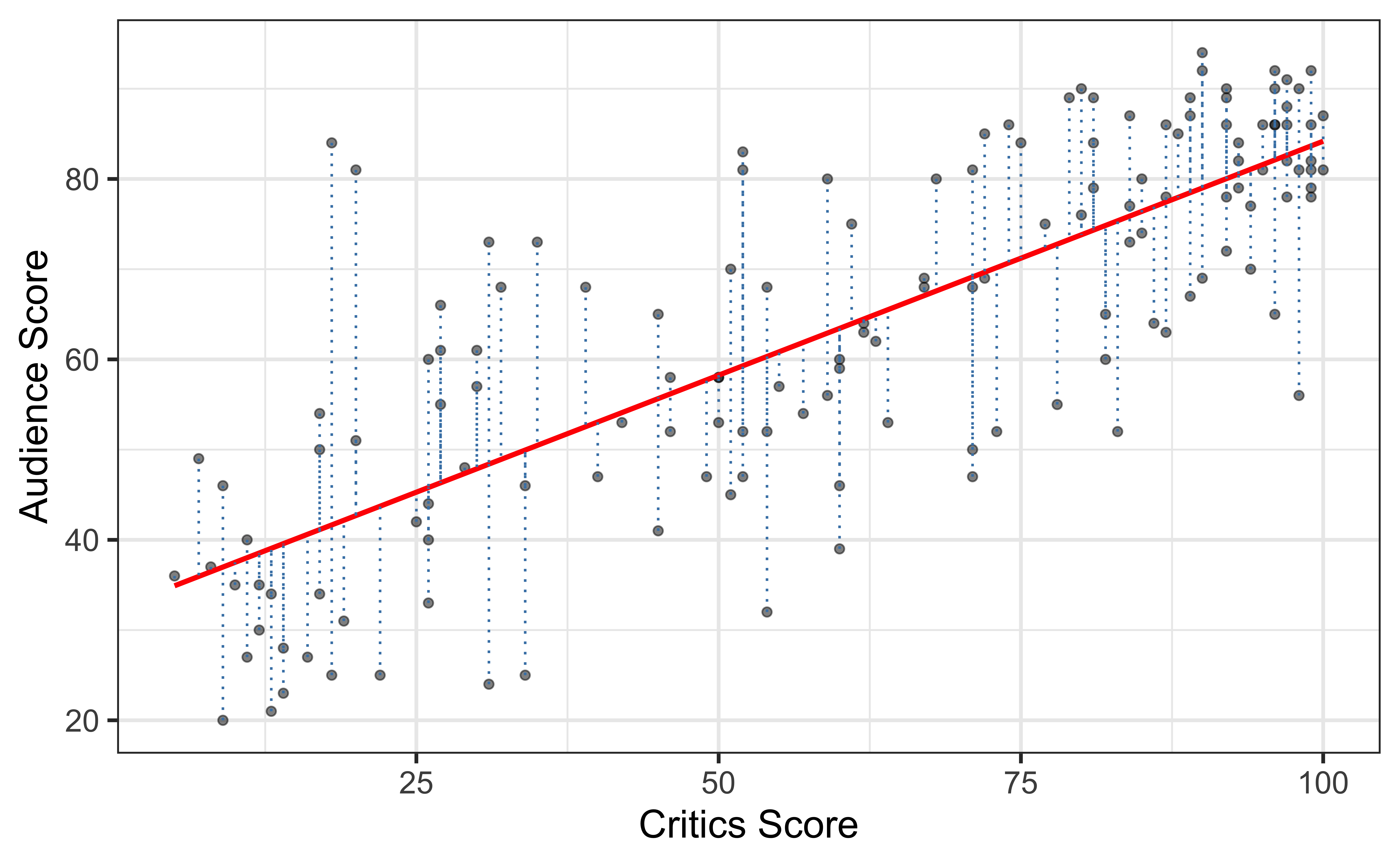

\[\text{residual} = \text{observed} - \text{predicted} = y_i - \hat{y}_i\]

Least squares line

The residual for the \(i^{th}\) observation is

\[e_i = \text{observed} - \text{predicted} = y_i - \hat{y}_i\]

The sum of squared residuals is

\[e^2_1 + e^2_2 + \dots + e^2_n\]

The least squares line is the one that minimizes the sum of squared residuals

Slope and intercept

Properties of least squares regression

The regression line goes through the center of mass point, the coordinates corresponding to average \(X\) and average \(Y\): \(\hat{\beta}_0 = \bar{Y} - \hat{\beta}_1\bar{X}\)
The slope has the same sign as the correlation coefficient: \(\hat{\beta}_1 = r \frac{s_Y}{s_X}\)
The sum of the residuals is approximately zero: \(\sum_{i = 1}^n e_i \approx 0\)
The residuals and \(X\) values are uncorrelated

Estimating the slope

\[\large{\hat{\beta}_1 = r \frac{s_Y}{s_X}}\]

\[\begin{aligned} s_X &= 30.1688 \\ s_Y &= 20.0244 \\ r &= 0.7814 \end{aligned}\]

\[\begin{aligned} \hat{\beta}_1 &= 0.7814 \times \frac{20.0244}{30.1688} \\ &= 0.5187\end{aligned}\]

Clickhere for details on deriving the equations for slope and intercept.

Estimating the intercept

\[\large{\hat{\beta}_0 = \bar{Y} - \hat{\beta}_1\bar{X}}\]

\[\begin{aligned} &\bar{x} = 60.8493 \\ &\bar{y} = 63.8767 \\ &\hat{\beta}_1 = 0.5187 \end{aligned}\]

\[\begin{aligned}\hat{\beta}_0 &= 63.8767 - 0.5187 \times 60.8493 \\ &= 32.3142 \end{aligned}\]

Click here for details on deriving the equations for slope and intercept.

Interpretation

Post your answers to the following questions on Ed Discussion:

The slope of the model for predicting audience score from critics score is 0.5187 . Which of the following is the best interpretation of this value?
32.3142 is the predicted mean audience score for what type of movies?

Link for Section 001 (10:05am lecture)
Link for Section 002 (1:25pm lecture)

03:00

Does it make sense to interpret the intercept?

✅ The intercept is meaningful in the context of the data if

the predictor can feasibly take values equal to or near zero, or
there are values near zero in the observed data.

🛑 Otherwise, the intercept may not be meaningful!

Prediction

Making a prediction

Suppose that a movie has a critics score of 70. According to this model, what is the movie’s predicted audience score?

\[\begin{aligned} \widehat{\text{audience}} &= 32.3142 + 0.5187 \times \text{critics} \\ &= 32.3142 + 0.5187 \times 70 \\ &= 68.6232 \end{aligned}\]

Fitting regression models with tidymodels

tidymodels

The tidymodels framework is a collection of packages for modeling and machine learning using tidyverse principles.

library(tidymodels)

── Attaching packages ────────────────────────────────────── tidymodels 1.1.0 ──

✔ broom        1.0.5     ✔ rsample      1.1.1
✔ dials        1.2.0     ✔ tune         1.1.1
✔ infer        1.0.4     ✔ workflows    1.1.3
✔ modeldata    1.1.0     ✔ workflowsets 1.0.1
✔ parsnip      1.1.0     ✔ yardstick    1.2.0
✔ recipes      1.0.6

── Conflicts ───────────────────────────────────────── tidymodels_conflicts() ──
✖ scales::discard() masks purrr::discard()
✖ dplyr::filter()   masks stats::filter()
✖ recipes::fixed()  masks stringr::fixed()
✖ dplyr::lag()      masks stats::lag()
✖ yardstick::spec() masks readr::spec()
✖ recipes::step()   masks stats::step()
• Dig deeper into tidy modeling with R at https://www.tmwr.org

Why tidymodels?

Consistent syntax for different model types (linear, logistic, random forest, Bayesian, etc.)
Streamline modeling workflow
- Split data into train and test sets
- Transform and create new variables
- Assess model performance
- Use model for prediction and inference

Fitting the model

Step 1: Specify model

linear_reg()

Linear Regression Model Specification (regression)

Computational engine: lm

Step 2: Set model fitting engine

linear_reg() |>
  set_engine("lm") # lm: linear model

Linear Regression Model Specification (regression)

Computational engine: lm

Step 3: Fit model & estimate parameters

using formula syntax

linear_reg() |>
  set_engine("lm") |>
  fit(audience ~ critics, data = movie_scores)

parsnip model object


Call:
stats::lm(formula = audience ~ critics, data = data)

Coefficients:
(Intercept)      critics  
    32.3155       0.5187

A closer look at the regression output

movie_fit <- linear_reg() |>
  set_engine("lm") |>
  fit(audience ~ critics, data = movie_scores)

movie_fit

parsnip model object


Call:
stats::lm(formula = audience ~ critics, data = data)

Coefficients:
(Intercept)      critics  
    32.3155       0.5187

\[\widehat{\text{audience}} = 32.3155 + 0.5187 \times \text{critics}\]

Note: The intercept is off by a tiny bit from the hand-calculated intercept, this is just due to rounding in the hand calculation.

The regression output

We’ll focus on the first column for now…

linear_reg() |>
  set_engine("lm") |>
  fit(audience ~ critics, data = movie_scores) |>
  tidy()

# A tibble: 2 × 5
  term        estimate std.error statistic  p.value
  <chr>          <dbl>     <dbl>     <dbl>    <dbl>
1 (Intercept)   32.3      2.34        13.8 4.03e-28
2 critics        0.519    0.0345      15.0 2.70e-31

Format output with `kable`

Use the kable function from the knitr package to produce a table and specify number of significant digits

linear_reg() |>
  set_engine("lm") |>
  fit(audience ~ critics, data = movie_scores) |>
  tidy() |>
  kable(digits = 4)

term	estimate	std.error	statistic	p.value
(Intercept)	32.3155	2.3425	13.7953	0
critics	0.5187	0.0345	15.0281	0

Prediction

# create a data frame for a new movie
new_movie <- tibble(critics = 70)

# predict the outcome for a new movie
predict(movie_fit, new_movie)

# A tibble: 1 × 1
  .pred
  <dbl>
1  68.6

Application exercise

📋 sta210-fa23.netlify.app/ae/ae-03-slr.html

Find your ae-03 repo in the course GitHub organization.
If you do not see an ae-03 repo, click here to create one.

Wrap up

Recap

Used simple linear regression to describe the relationship between a quantitative predictor and quantitative response variable.
Used the least squares method to estimate the slope and intercept.
Interpreted the slope and intercept.
- Slope: For every one unit increase in \(x\), we expect y to change by \(\hat{\beta}_1\) units, on average.
- Intercept: If \(x\) is 0, then we expect \(y\) to be \(\hat{\beta}_0\) units
Predicted the response given a value of the predictor variable.
Used tidymodels to fit and summarize regression models in R.

Simple Linear Regression

Questions?

Join sta210-fa23 on GitHub

Topics

Computation set up

Data

Movie scores

Data prep

Data overview

Movie scores data

Movie ratings data

Why fit a line?

Terminology

Regression model

Regression model

Regression model

Simple linear regression (SLR)

SLR: Statistical model

SLR: Regression equation

Choosing values for \(\hat{\beta}_1\) and \(\hat{\beta}_0\)

Residuals

Least squares line

Slope and intercept

Properties of least squares regression

Estimating the slope

Estimating the intercept

Interpretation

Does it make sense to interpret the intercept?

Prediction

Making a prediction

Fitting regression models with tidymodels

tidymodels

Why tidymodels?

Fitting the model

Step 1: Specify model

Step 2: Set model fitting engine

Step 3: Fit model & estimate parameters

A closer look at the regression output

The regression output

Format output with kable

Prediction

Application exercise

Wrap up

Recap

Format output with `kable`