AE 03: Bike rentals in Washington, DC

Simple linear regression

Important

Go to the course GitHub organization and locate your ae-03 repo to get started. If you do not see an ae-03 repo, click here to create one.

Render, commit, and push your responses to GitHub by the end of class. The responses are due in your GitHub repo no later than Saturday, September 9 at 11:59pm.

library(tidyverse)
library(tidymodels)
library(patchwork)

Data

Our data set contains daily rentals from the Capital Bikeshare in Washington, DC in 2011 and 2012. It was obtained from the dcbikeshare data set in the dsbox R package.

We will focus on the following variables in the analysis:

• count: total bike rentals
• temp_orig: Temperature in degrees Celsius
• season: 1 - winter, 2 - spring, 3 - summer, 4 - fall

Click here for the full list of variables and definitions.

bikeshare <- read_csv("data/dcbikeshare.csv")

Exercises

Exercise 1

Below are visualizations of the distributions of daily bike rentals and temperature as well as the relationship between these two variables.

p1 <- ggplot(bikeshare, aes(x = count)) +
  geom_histogram(binwidth = 250) + 
  labs(x = "Daily bike rentals")

p2 <- ggplot(bikeshare, aes(x = temp_orig)) +
  geom_histogram() + 
  labs(x = "Temperature (Celsius)")

p3 <- ggplot(bikeshare, aes(y = count, x = temp_orig)) +
  geom_point() + 
  labs(x = "Temperature (Celsius)", 
       y = "Daily bike rentals")

(p1 | p2) / p3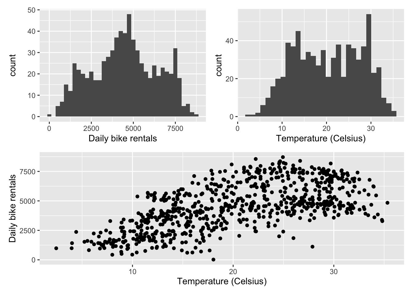

There appears to be one day with a very small number of bike rentals. What was the day? Why were the number of bike rentals so low on that day? Hint: You can Google the date to figure out what was going on that day.

[Add your answer here]

Exercise 2

In the raw data, seasons are coded as 1, 2, 3, 4 as numerical values, corresponding to winter, spring, summer, and fall respectively. Recode the season variable to make it a categorical variable (a factor) with levels corresponding to season names, making sure that the levels appear in a reasonable order in the variable (i.e., not alphabetical).

# add code developed during livecoding here

Exercise 3

We want to evaluate whether the relationship between temperature and daily bike rentals is the same for each season. To answer this question, first create a scatter plot of daily bike rentals vs. temperature faceted by season.

# add code developed during livecoding here

Exercise 4

• Which season appears to have the strongest relationship between temperature and daily bike rentals? Why do you think the relationship is strongest in this season?

• Which season appears to have the weakest relationship between temperature and daily bike rentals? Why do you think the relationship is weakest in this season?

[Add your answer here]

Exercise 5

Filter your data for the season with the strongest apparent relationship between temperature and daily bike rentals.

# add code developed during livecoding here

Exercise 6

Using the subset of the data from Exercise 5, fit a linear model for predicting daily bike rentals from temperature for this season.

# add code developed during livecoding here

Exercise 7

Use the output to write out the estimated regression equation.

[Add your answer here]

Exercise 8

Interpret the slope in the context of the data.

[Add your answer here]

Exercise 9

Interpret the intercept in the context of the data.

[Add your answer here]

Exercise 10

Suppose you work for a bike share company in Durham, NC, and they want to predict daily bike rentals in 2024. What is one reason you might recommend they use your analysis for this task? What is one reason you would recommend they not use your analysis for this task?

[Add your answer here]

---

Important

To submit the AE:

• Render the document to produce the PDF with all of your work from today’s class.
• Push all your work to your ae-03- repo on GitHub. (You do not submit AEs on Gradescope).