Multinomial logistic regression

Prediction + inference

Prof. Maria Tackett

Nov 27, 2023

Announcements

• Due dates

  • HW 05 due Wed, Nov 29 at 11:59pm

• Project

  • (Optional) Round 1 submission due Fri, Dec 01 at 11:59pm
  • Presentations in lab Dec 5 & 7

• Exam 02 dates

  • In-class: Mon, Dec 4
  • Take-home: Mon, Dec 4 - Wed, Dec 6
  • Review: Wed, Nov 29

• Click here to access lecture recordings. Available until Mon, Dec 04 at 9am

Statistician of the day: Mike Dairyko

Mike Dairyko was a student at Pomona College where he studied Mathematics. Through a linear algebra class, he found his way to two different summer REU programs and eventually to a PhD in Applied Mathematics from Iowa State University (2018). Being introduced to machine learning methods caused him to pursue data science jobs after graduation.

Dr. Dairyko served as a Senior Manager of Data Science at the Milwaukee Brewers and is now the Director of Ticketing Analytics at the Milwaukee Bucks. Helping the organization get the most out of budgeting, revenue, and ticket sales allows him to fully use his training in mathematics and data science.

Source: hardin47.github.io/CURV/scholars/dairyko

Statistician of the day

About his role as a Senior Manager of Data Science for the MilwaukeeBrewers:

“During the season, one of my main priorities is to produce game-by-game ticket and revenue projections. To do so, my group incorporates historical data—such as team performance, weather, and schedules—into multiple regression-based models and then consolidates the outputs in an easily-digestible format. A large codebase both automates and maintains this process; the codebase is regularly tweaked to ensure that it is agile enough to handle the constant usage and flow of new information.”

“Our projections are most accurate when we utilize both qualitative and quantitative forecasts.”

Source: From Academia to Major League Baseball: The Journey of a Data Scientist

Statistician of the day

About his role as a Senior Manager of Data Science for the Milwaukee Brewers:

“Mathematicians are ultimately trained to develop problem-solving skills and apply them with persistence and creativity…Carefully reviewing the work—and perhaps redoing it a different way or approaching the issue from another angle—eventually leads to success…I do use the problem-solving strategies, persistence, and creativity that I have honed throughout my mathematical journey every single day.”

“I would encourage students to become comfortable with navigating a programming language such as R or Python…Briefly stepping outside of mathematics and establishing computer science and statistics expertise is also useful…Finally, participating in conferences with data science content is an excellent way to gain exposure to more advanced topics in the field and build a network within the community.”

Source: From Academia to Major League Baseball: The Journey of a Data Scientist

Topics

• Predictions
• Model selection
• Checking conditions

Computational setup

# load packages
library(tidyverse)
library(tidymodels)
library(NHANES)
library(knitr)
library(patchwork)
library(colorblindr)
library(pROC)
library(Stat2Data)
library(nnet)

# set default theme and larger font size for ggplot2
ggplot2::theme_set(ggplot2::theme_minimal(base_size = 20))

NHANES Data

• National Health and Nutrition Examination Survey is conducted by the National Center for Health Statistics (NCHS).
• The goal is to “assess the health and nutritional status of adults and children in the United States”.
• This survey includes an interview and a physical examination.

Variables

Goal: Use a person’s age and whether they do regular physical activity to predict their self-reported health rating.

• Outcome: HealthGen: Self-reported rating of participant’s health in general. Excellent, Vgood, Good, Fair, or Poor.

• Predictors:

  • Age: Age at time of screening (in years). Participants 80 or older were recorded as 80.
  • PhysActive: Participant does moderate to vigorous-intensity sports, fitness or recreational activities.

The data

nhanes_adult <- NHANES |>
  filter(Age >= 18) |>
  select(HealthGen, Age, PhysActive, Education) |>
  drop_na() |>
  mutate(obs_num = 1:n())

glimpse(nhanes_adult)

Rows: 6,465
Columns: 5
$ HealthGen  <fct> Good, Good, Good, Good, Vgood, Vgood, Vgood, Vgood, Vgood, …
$ Age        <int> 34, 34, 34, 49, 45, 45, 45, 66, 58, 54, 50, 33, 60, 56, 56,…
$ PhysActive <fct> No, No, No, No, Yes, Yes, Yes, Yes, Yes, Yes, Yes, No, No, …
$ Education  <fct> High School, High School, High School, Some College, Colleg…
$ obs_num    <int> 1, 2, 3, 4, 5, 6, 7, 8, 9, 10, 11, 12, 13, 14, 15, 16, 17, …

Model in R

health_fit <- multinom_reg() |>
  set_engine("nnet") |>
  fit(HealthGen ~ Age + PhysActive, data = nhanes_adult)

Model summary

tidy(health_fit) |> kable(digits = 3)

y.level	term	estimate	std.error	statistic	p.value
Vgood	(Intercept)	1.265	0.154	8.235	0.000
Vgood	Age	0.000	0.003	-0.014	0.989
Vgood	PhysActiveYes	-0.332	0.095	-3.496	0.000
Good	(Intercept)	1.989	0.150	13.285	0.000
Good	Age	-0.003	0.003	-1.187	0.235
Good	PhysActiveYes	-1.011	0.092	-10.979	0.000
Fair	(Intercept)	1.033	0.174	5.938	0.000
Fair	Age	0.001	0.003	0.373	0.709
Fair	PhysActiveYes	-1.662	0.109	-15.190	0.000
Poor	(Intercept)	-1.338	0.299	-4.475	0.000
Poor	Age	0.019	0.005	3.827	0.000
Poor	PhysActiveYes	-2.670	0.236	-11.308	0.000

Predictions

Calculating probabilities

• Suppose the repsonse variable has \(K\) categories and \(k = 1\) is the baseline category. For categories \(2,\ldots,K\), the probability that the \(i^{th}\) observation is in the \(j^{th}\) category is

  \[ \hat{\pi}_{ij} = \frac{\exp\{\hat{\beta}_{0j} + \hat{\beta}_{1j}x_{i1} + \dots + \hat{\beta}_{pj}x_{ip}\}}{1 + \sum\limits_{k=2}^K \exp\{\hat{\beta}_{0k} + \hat{\beta}_{1k}x_{i1} + \dots \hat{\beta}_{pk}x_{ip}\}} \]

• For the baseline category, \(k=1\), we calculate the probability \(\hat{\pi}_{i1}\) as

  \[ \hat{\pi}_{i1} = 1- \sum\limits_{k=2}^K \hat{\pi}_{ik} \]

Predicted health rating

We can use our model to predict a person’s perceived health rating given their age and whether they exercise.

health_aug <- augment(health_fit, new_data = nhanes_adult)
health_aug

# A tibble: 6,465 × 11
   .pred_class .pred_Excellent .pred_Vgood .pred_Good .pred_Fair .pred_Poor
   <fct>                 <dbl>       <dbl>      <dbl>      <dbl>      <dbl>
 1 Good                 0.0687       0.243      0.453     0.201     0.0348 
 2 Good                 0.0687       0.243      0.453     0.201     0.0348 
 3 Good                 0.0687       0.243      0.453     0.201     0.0348 
 4 Good                 0.0691       0.244      0.435     0.205     0.0467 
 5 Vgood                0.155        0.393      0.359     0.0868    0.00671
 6 Vgood                0.155        0.393      0.359     0.0868    0.00671
 7 Vgood                0.155        0.393      0.359     0.0868    0.00671
 8 Vgood                0.157        0.400      0.342     0.0904    0.0102 
 9 Vgood                0.156        0.397      0.349     0.0890    0.00872
10 Vgood                0.156        0.396      0.352     0.0883    0.00804
# ℹ 6,455 more rows
# ℹ 5 more variables: HealthGen <fct>, Age <int>, PhysActive <fct>,
#   Education <fct>, obs_num <int>

Actual vs. predicted health rating

For each observation, the predicted perceived health rating is the category with the highest predicted probability.

health_aug |> select(contains("pred"))

# A tibble: 6,465 × 6
   .pred_class .pred_Excellent .pred_Vgood .pred_Good .pred_Fair .pred_Poor
   <fct>                 <dbl>       <dbl>      <dbl>      <dbl>      <dbl>
 1 Good                 0.0687       0.243      0.453     0.201     0.0348 
 2 Good                 0.0687       0.243      0.453     0.201     0.0348 
 3 Good                 0.0687       0.243      0.453     0.201     0.0348 
 4 Good                 0.0691       0.244      0.435     0.205     0.0467 
 5 Vgood                0.155        0.393      0.359     0.0868    0.00671
 6 Vgood                0.155        0.393      0.359     0.0868    0.00671
 7 Vgood                0.155        0.393      0.359     0.0868    0.00671
 8 Vgood                0.157        0.400      0.342     0.0904    0.0102 
 9 Vgood                0.156        0.397      0.349     0.0890    0.00872
10 Vgood                0.156        0.396      0.352     0.0883    0.00804
# ℹ 6,455 more rows

Confusion matrix

health_conf <- health_aug |> 
  count(HealthGen, .pred_class, .drop = FALSE) |>
  pivot_wider(names_from = .pred_class, values_from = n)

health_conf

# A tibble: 5 × 6
  HealthGen Excellent Vgood  Good  Fair  Poor
  <fct>         <int> <int> <int> <int> <int>
1 Excellent         0   528   210     0     0
2 Vgood             0  1341   743     0     0
3 Good              0  1226  1316     0     0
4 Fair              0   296   625     0     0
5 Poor              0    24   156     0     0

Actual vs. predicted health rating

Why do you think no observations were predicted to have a rating of “Excellent”, “Fair”, or “Poor”?

ROC curves

ROC curves for multiclass outcomes use a one-vs-all approach: calculate multiple curves, one per level vs. all other levels.

health_aug |> 
  roc_curve(
    truth = HealthGen, 
    .pred_Excellent:.pred_Poor
  ) |> 
  autoplot()

ROC curves

ROC curve: under the hood

An additional column, .level, identifies the “one” column in the one-vs-all calculation:

health_aug |> 
  roc_curve(
    truth = HealthGen, 
    .pred_Excellent:.pred_Poor
  )

# A tibble: 620 × 4
   .level    .threshold specificity sensitivity
   <chr>          <dbl>       <dbl>       <dbl>
 1 Excellent  -Inf          0             1    
 2 Excellent     0.0681     0             1    
 3 Excellent     0.0682     0.00664       0.997
 4 Excellent     0.0682     0.0138        0.992
 5 Excellent     0.0683     0.0192        0.989
 6 Excellent     0.0683     0.0243        0.981
 7 Excellent     0.0684     0.0297        0.970
 8 Excellent     0.0684     0.0353        0.969
 9 Excellent     0.0684     0.0426        0.951
10 Excellent     0.0685     0.0492        0.947
# ℹ 610 more rows

Model selection for inference

Comparing nested models

• Suppose there are two models:
  • Reduced model includes predictors \(x_1, \ldots, x_q\)
  • Full model includes predictors \(x_1, \ldots, x_q, x_{q+1}, \ldots, x_p\)
• We want to test the following hypotheses:
  • \(H_0: \beta_{q+1} = \dots = \beta_p = 0\)
  • \(H_A: \text{ at least 1 }\beta_j \text{ is not } 0\)
• To do so, we will use the drop-in-deviance test (very similar to logistic regression)

Add Education to the model?

• We consider adding the participants’ Education level to the model.
  • Education takes values 8thGrade, 9-11thGrade, HighSchool, SomeCollege, and CollegeGrad
• Models we’re testing:
  • Reduced model: Age, PhysActive
  • Full model: Age, PhysActive, Education

\[ \begin{align} &H_0: \beta_{9-11thGrade} = \beta_{HighSchool} = \beta_{SomeCollege} = \beta_{CollegeGrad} = 0\\ &H_a: \text{ at least one }\beta_j \text{ is not equal to }0 \end{align} \]

Add Education to the model?

reduced_fit <- multinom_reg() |>
  set_engine("nnet") |>
  fit(HealthGen ~ Age + PhysActive,
  data = nhanes_adult)

full_fit <- multinom_reg() |>
  set_engine("nnet") |>
  fit(HealthGen ~ Age + PhysActive + Education,
  data = nhanes_adult)

Add Education to the model?

anova(reduced_fit$fit, full_fit$fit, test = "Chisq") |>
  kable(digits = 3)

Model	Resid. df	Resid. Dev	Test	Df	LR stat.	Pr(Chi)
Age + PhysActive	25848	16994.23		NA	NA	NA
Age + PhysActive + Education	25832	16505.10	1 vs 2	16	489.132	0

At least one coefficient associated with Education is non-zero. Therefore, we will include Education in the model.

Model with Education

tidy(full_fit, conf.int = T) |> print(n = 28) 

# A tibble: 28 × 8
   y.level term         estimate std.error statistic  p.value conf.low conf.high
   <chr>   <chr>           <dbl>     <dbl>     <dbl>    <dbl>    <dbl>     <dbl>
 1 Vgood   (Intercept)   5.82e-1   0.301      1.93   5.36e- 2 -0.00914   1.17   
 2 Vgood   Age           1.12e-3   0.00266    0.419  6.75e- 1 -0.00411   0.00634
 3 Vgood   PhysActiveY… -2.64e-1   0.0985    -2.68   7.33e- 3 -0.457    -0.0711 
 4 Vgood   Education9 …  7.68e-1   0.308      2.49   1.27e- 2  0.164     1.37   
 5 Vgood   EducationHi…  7.01e-1   0.280      2.51   1.21e- 2  0.153     1.25   
 6 Vgood   EducationSo…  7.88e-1   0.271      2.90   3.71e- 3  0.256     1.32   
 7 Vgood   EducationCo…  4.08e-1   0.268      1.52   1.28e- 1 -0.117     0.933  
 8 Good    (Intercept)   2.04e+0   0.272      7.51   5.77e-14  1.51      2.57   
 9 Good    Age          -1.72e-3   0.00263   -0.651  5.15e- 1 -0.00688   0.00345
10 Good    PhysActiveY… -7.58e-1   0.0961    -7.88   3.16e-15 -0.946    -0.569  
11 Good    Education9 …  3.60e-1   0.275      1.31   1.90e- 1 -0.179     0.899  
12 Good    EducationHi…  8.52e-2   0.247      0.345  7.30e- 1 -0.399     0.569  
13 Good    EducationSo… -1.13e-2   0.239     -0.0472 9.62e- 1 -0.480     0.457  
14 Good    EducationCo… -8.91e-1   0.236     -3.77   1.65e- 4 -1.35     -0.427  
15 Fair    (Intercept)   2.12e+0   0.288      7.35   1.91e-13  1.55      2.68   
16 Fair    Age           3.35e-4   0.00312    0.107  9.14e- 1 -0.00578   0.00645
17 Fair    PhysActiveY… -1.19e+0   0.115    -10.4    3.50e-25 -1.42     -0.966  
18 Fair    Education9 … -2.24e-1   0.279     -0.802  4.22e- 1 -0.771     0.323  
19 Fair    EducationHi… -8.32e-1   0.252     -3.31   9.44e- 4 -1.33     -0.339  
20 Fair    EducationSo… -1.34e+0   0.246     -5.46   4.71e- 8 -1.82     -0.861  
21 Fair    EducationCo… -2.51e+0   0.253     -9.91   3.67e-23 -3.00     -2.01   
22 Poor    (Intercept)  -2.00e-1   0.411     -0.488  6.26e- 1 -1.01      0.605  
23 Poor    Age           1.79e-2   0.00509    3.53   4.21e- 4  0.00797   0.0279 
24 Poor    PhysActiveY… -2.27e+0   0.242     -9.38   6.81e-21 -2.74     -1.79   
25 Poor    Education9 … -3.60e-1   0.353     -1.02   3.08e- 1 -1.05      0.332  
26 Poor    EducationHi… -1.15e+0   0.334     -3.44   5.86e- 4 -1.81     -0.494  
27 Poor    EducationSo… -1.07e+0   0.316     -3.40   6.77e- 4 -1.69     -0.454  
28 Poor    EducationCo… -2.32e+0   0.366     -6.34   2.27e-10 -3.04     -1.60   

Compare models using AIC & BIC

AIC

Reduced model:

glance(reduced_fit)$AIC

[1] 17018.23

Full model:

glance(full_fit)$AIC

[1] 16561.1

BIC

Reduced model:

glance(reduced_fit)$deviance + log(nrow(nhanes_adult)) * glance(reduced_fit)$edf

[1] 17099.52

Full model:

glance(full_fit)$deviance + log(nrow(nhanes_adult)) * glance(full_fit)$edf

[1] 16750.77

Checking conditions for inference

Conditions for inference

We want to check the following conditions for inference for the multinomial logistic regression model:

1. Linearity: Is there a linear relationship between the log-odds and the predictor variables?

2. Randomness: Was the sample randomly selected? Or can we reasonably treat it as random?

3. Independence: Are the observations independent?

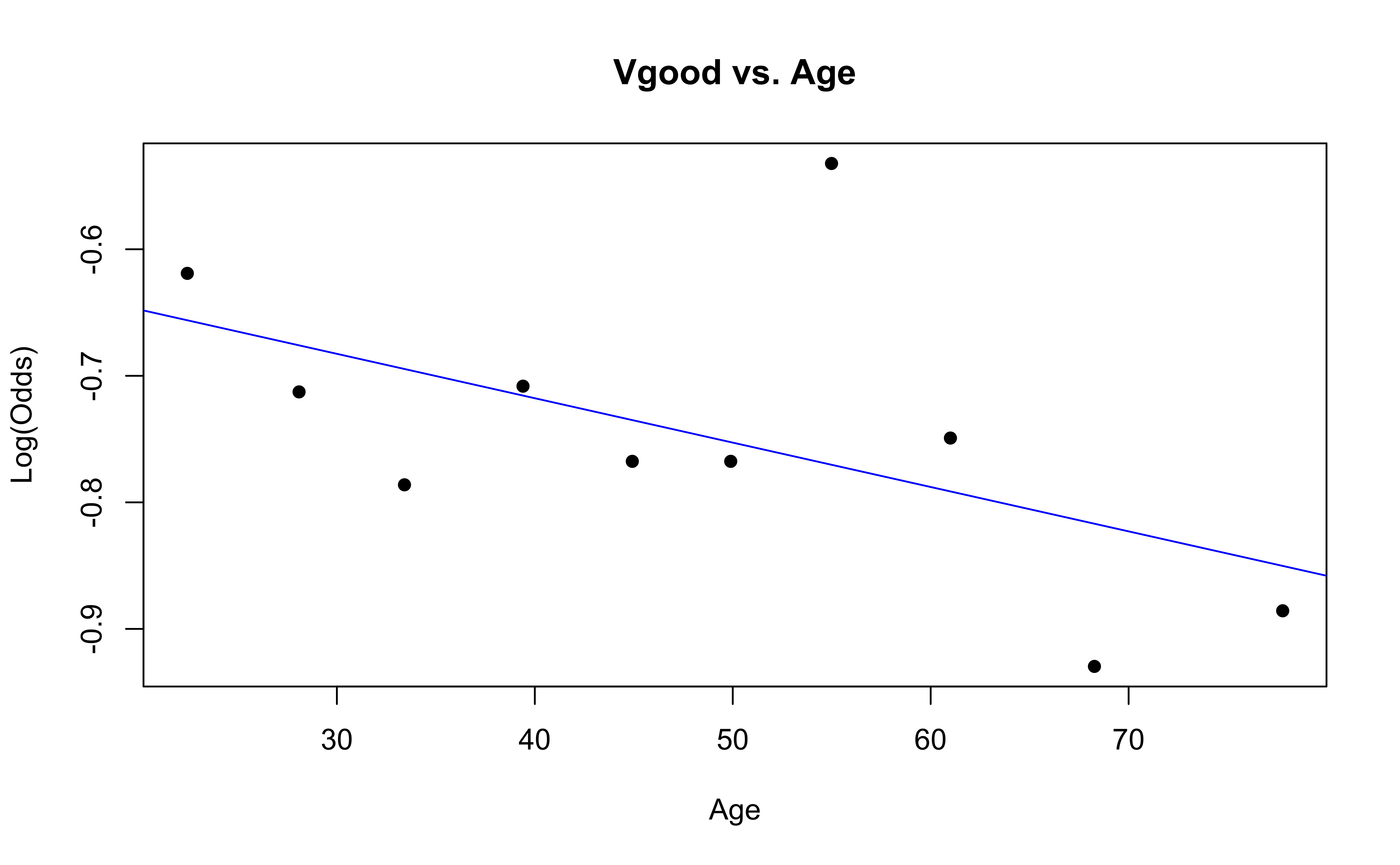
Checking linearity

Similar to logistic regression, we will check linearity by examining empirical logit plots between each level of the response and the quantitative predictor variables.

nhanes_adult <- nhanes_adult |>
  mutate(
    Excellent = factor(if_else(HealthGen == "Excellent", "1", "0")),
    Vgood = factor(if_else(HealthGen == "Vgood", "1", "0")),
    Good = factor(if_else(HealthGen == "Good", "1", "0")),
    Fair = factor(if_else(HealthGen == "Fair", "1", "0")),
    Poor = factor(if_else(HealthGen == "Poor", "1", "0"))
  )

Checking linearity

emplogitplot1(Excellent ~ Age, data = nhanes_adult, 
              ngroups = 10, main = "Excellent vs. Age")
emplogitplot1(Vgood ~ Age, data = nhanes_adult, 
              ngroups = 10, main = "Vgood vs. Age")

Checking linearity

emplogitplot1(Good ~ Age, data = nhanes_adult, 
              ngroups = 10, main = "Good vs. Age")
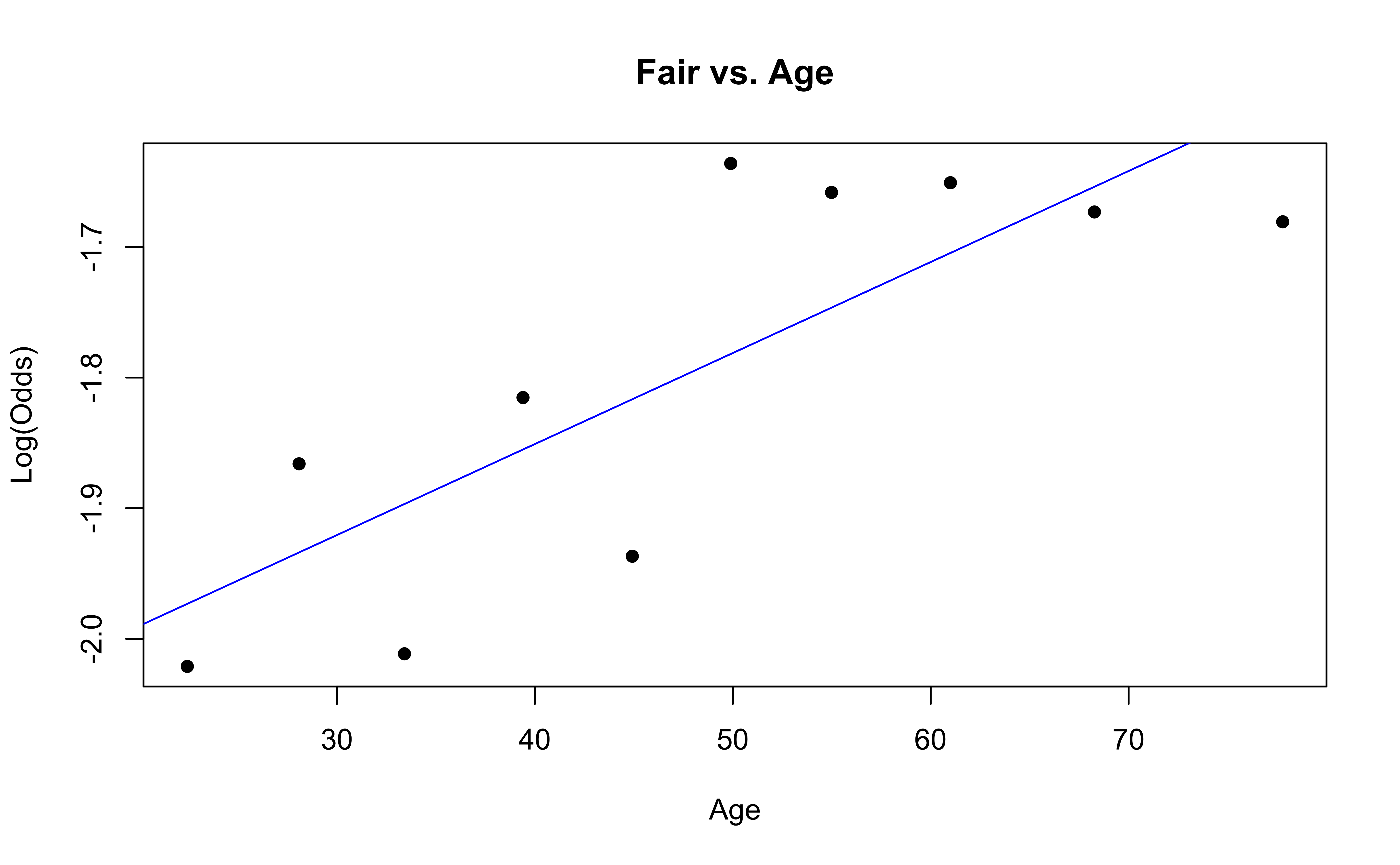
emplogitplot1(Fair ~ Age, data = nhanes_adult, 
              ngroups = 10, main = "Fair vs. Age")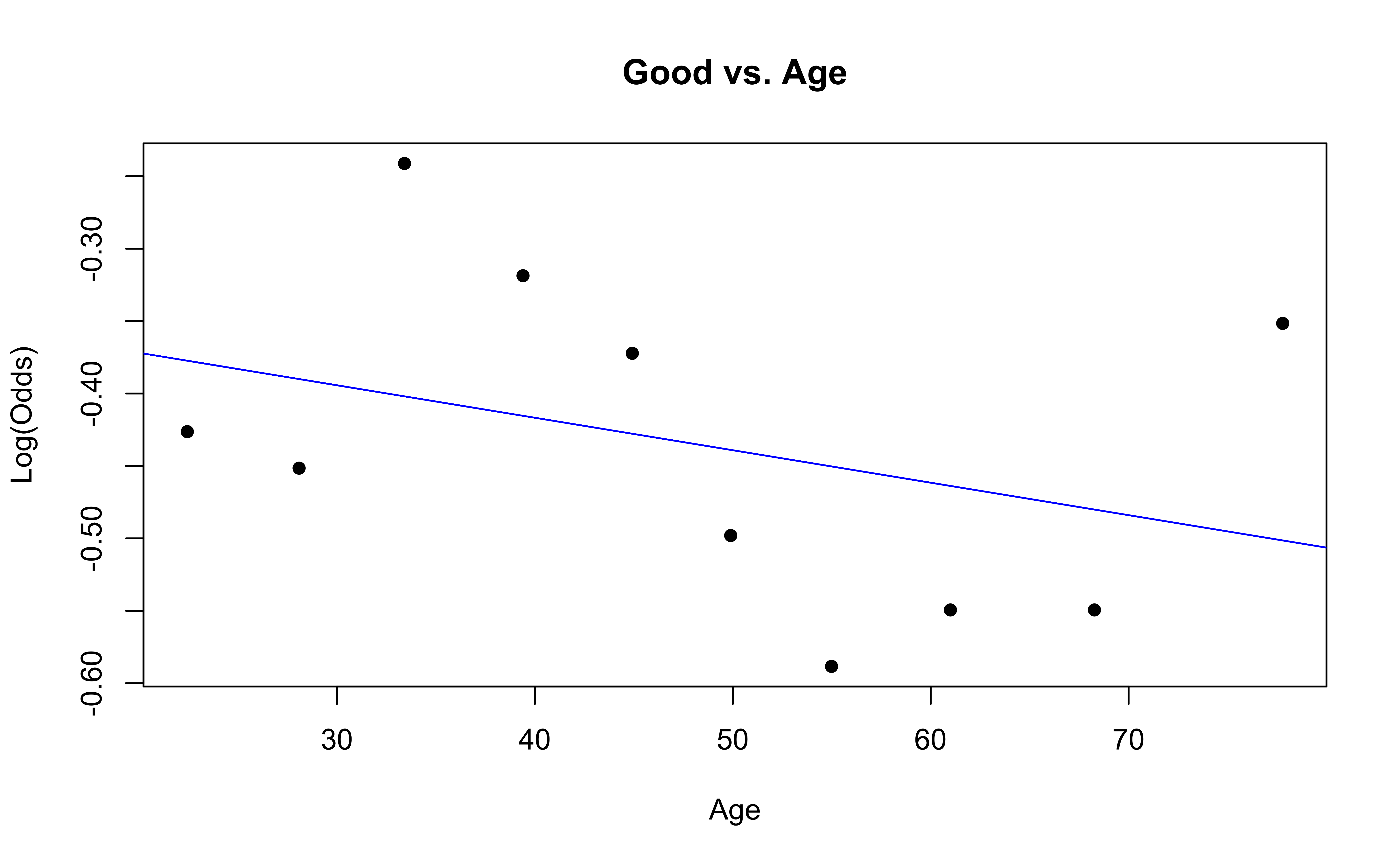

Checking linearity

emplogitplot1(Poor ~ Age, data = nhanes_adult, 
              ngroups = 10, main = "Poor vs. Age")

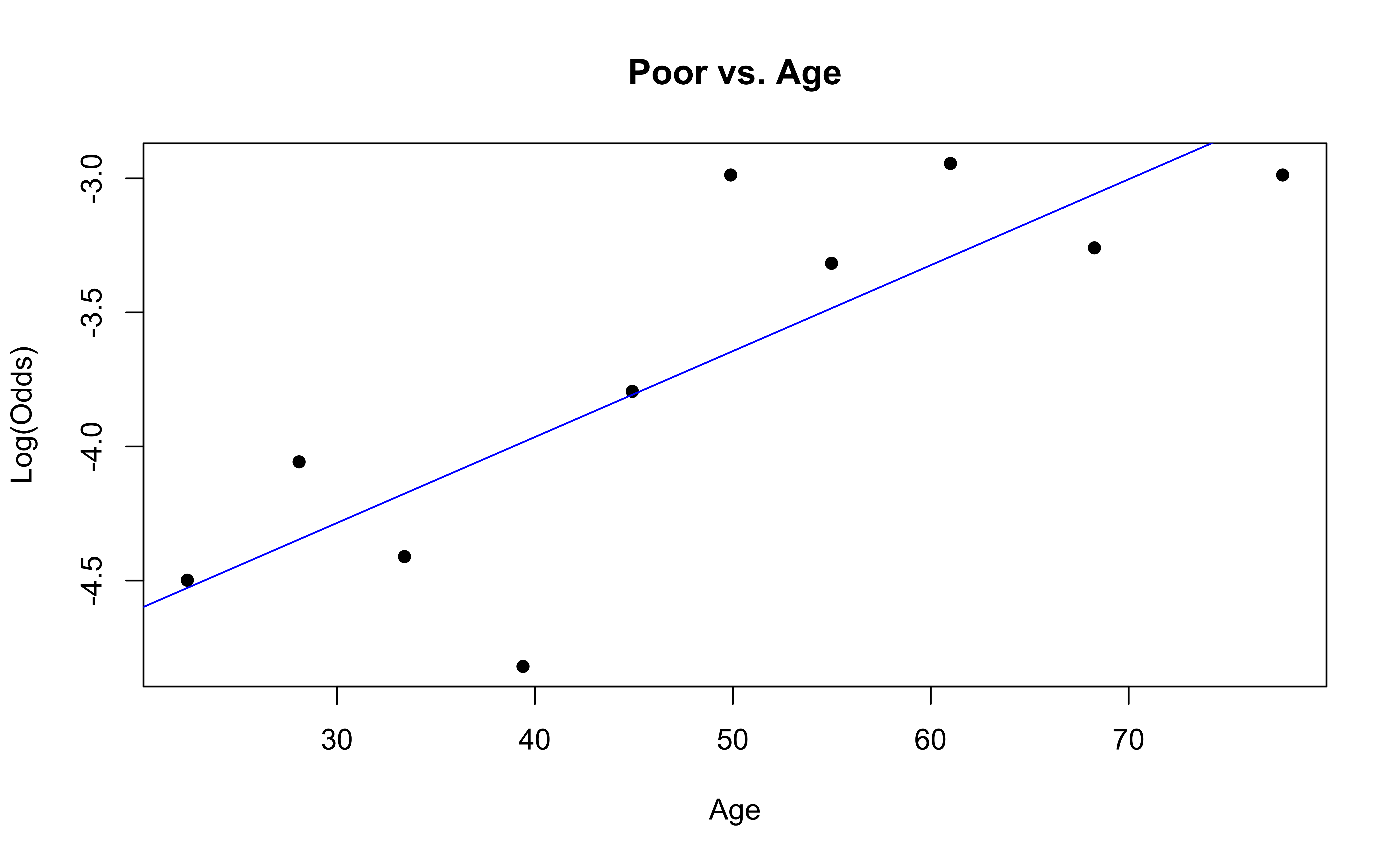
✅ The linearity condition is satisfied. There is generally a linear relationship between the empirical logit and the quantitative predictor variable, Age, for each level of the response.

Checking randomness

We can check the randomness condition based on the context of the data and how the observations were collected.

• Was the sample randomly selected?

• If the sample was not randomly selected, ask whether there is reason to believe the observations in the sample differ systematically from the population of interest.

✅ The randomness condition is satisfied. The participants were randomly selected, and thus we do not have reason to believe that the participants in this study differ systematically from adults in the U.S.

Checking independence

We can check the independence condition based on the context of the data and how the observations were collected.

Independence is most often violated if the data were collected over time or there is a strong spatial relationship between the observations.

✅ The independence condition is satisfied. The participants were randomly selected, so it is reasonable to conclude that the participants’ health and behavior characteristics are independent of one another.

Recap

• Predictions
• Model selection for inference
• Checking conditions for inference

Full multinomial modeling workflow

• juliasilge.com/blog/multinomial-volcano-eruptions

• juliasilge.com/blog/nber-papers

Questions for Exam 02 review

Submit your questions for the Exam 02 review: https://forms.office.com/r/cTyeRjVmfb

Exam 02 will cover multiple linear regression, logistic regression, and multinomial logistic regression.