Logistic Regression: Model comparison

Prof. Maria Tackett

Nov 08, 2023

Announcements

Project draft due in your GitHub repo at 9am on
- November 14 (Tuesday labs)
- November 16 (Thursday labs)
- Will do peer review in lab those days
Team Feedback #1 due Friday, November 10 at 11:5pm
- Received email from teammates
HW 04 due Wednesday, November 15 at 11:59pm
- Released later today

Topics

Comparing logistic regression models using

Drop-in-deviance test
AIC
BIC

Computational setup

# load packages
library(tidyverse)
library(tidymodels)
library(openintro)
library(knitr)
library(kableExtra)  # for table embellishments
library(Stat2Data)   # for empirical logit

# set default theme and larger font size for ggplot2
ggplot2::theme_set(ggplot2::theme_bw(base_size = 20))

Data

Risk of coronary heart disease

This data set is from an ongoing cardiovascular study on residents of the town of Framingham, Massachusetts. We want to examine the relationship between various health characteristics and the risk of having heart disease.

high_risk:
- 1: High risk of having heart disease in next 10 years
- 0: Not high risk of having heart disease in next 10 years
age: Age at exam time (in years)
education: 1 = Some High School, 2 = High School or GED, 3 = Some College or Vocational School, 4 = College
currentSmoker: 0 = nonsmoker, 1 = smoker

Data prep

heart_disease <- read_csv(here::here("slides", "data/framingham.csv")) |>
  select(age, education, TenYearCHD, totChol, currentSmoker) |>
  drop_na() |> #consider the limitations of doing this
  mutate(
    high_risk = as.factor(TenYearCHD),
    education = as.factor(education),
    currentSmoker = as.factor(currentSmoker)
  )

heart_disease

# A tibble: 4,086 × 6
     age education TenYearCHD totChol currentSmoker high_risk
   <dbl> <fct>          <dbl>   <dbl> <fct>         <fct>    
 1    39 4                  0     195 0             0        
 2    46 2                  0     250 0             0        
 3    48 1                  0     245 1             0        
 4    61 3                  1     225 1             1        
 5    46 3                  0     285 1             0        
 6    43 2                  0     228 0             0        
 7    63 1                  1     205 0             1        
 8    45 2                  0     313 1             0        
 9    52 1                  0     260 0             0        
10    43 1                  0     225 1             0        
# ℹ 4,076 more rows

Modeling risk of coronary heart disease

Using age and education:

risk_fit <- logistic_reg() |>
  set_engine("glm") |>
  fit(high_risk ~ age + education, 
      data = heart_disease, family = "binomial")

Model output

tidy(risk_fit, conf.int = TRUE) |> 
  kable(format = "markdown", digits = 3)

term	estimate	std.error	statistic	p.value	conf.low	conf.high
(Intercept)	-5.508	0.311	-17.692	0.000	-6.125	-4.904
age	0.076	0.006	13.648	0.000	0.065	0.087
education2	-0.245	0.113	-2.172	0.030	-0.469	-0.026
education3	-0.236	0.135	-1.753	0.080	-0.504	0.024
education4	-0.024	0.150	-0.161	0.872	-0.323	0.264

\[ \small{\log\Big(\frac{\hat{\pi}}{1-\hat{\pi}}\Big) = -5.508 + 0.076 ~ \text{age} - 0.245 ~ \text{ed2} - 0.236 ~ \text{ed3} - 0.024 ~ \text{ed4}} \]

Should we add currentSmoker to this model?

Comparing logistic regression models

Log likelihood

\[ \log L = \sum\limits_{i=1}^n[y_i \log(\hat{\pi}_i) + (1 - y_i)\log(1 - \hat{\pi}_i)] \]

Measure of how well the model fits the data
Higher values of \(\log L\) are better
Deviance = \(-2 \log L\)
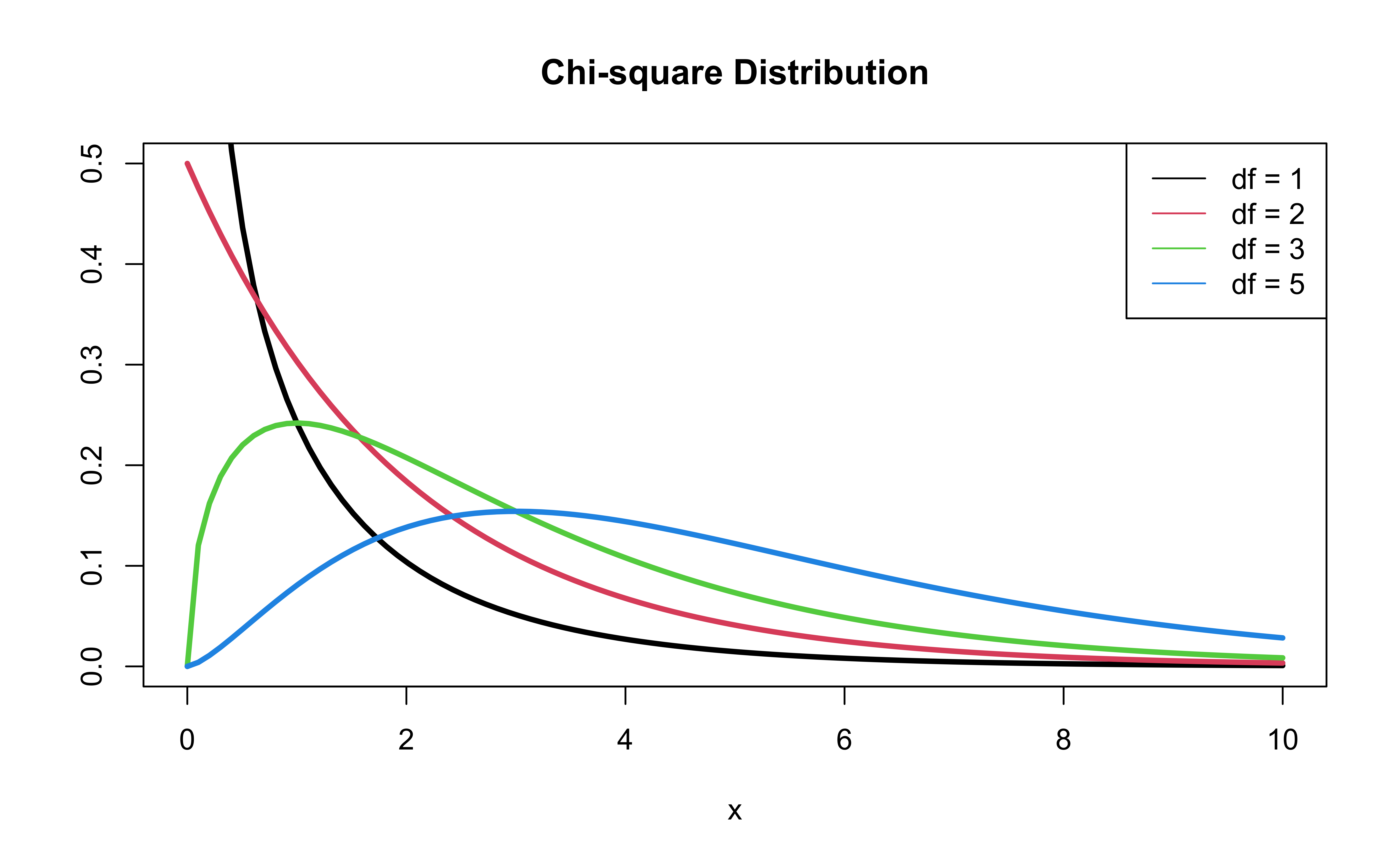
- \(-2 \log L\) follows a \(\chi^2\) distribution with \(n - p - 1\) degrees of freedom

Comparing nested models

Suppose there are two models:
- Reduced Model includes predictors \(x_1, \ldots, x_q\)
- Full Model includes predictors \(x_1, \ldots, x_q, x_{q+1}, \ldots, x_p\)
We want to test the hypotheses

\[ \begin{aligned} H_0&: \beta_{q+1} = \dots = \beta_p = 0 \\ H_A&: \text{ at least one }\beta_j \text{ is not } 0 \end{aligned} \]
To do so, we will use the Drop-in-deviance test, also known as the Nested Likelihood Ratio test

Drop-in-deviance test

Hypotheses:

\[ \begin{aligned} H_0&: \beta_{q+1} = \dots = \beta_p = 0 \\ H_A&: \text{ at least 1 }\beta_j \text{ is not } 0 \end{aligned} \]

Test Statistic: \[G = (-2 \log L_{reduced}) - (-2 \log L_{full})\]

P-value: \(P(\chi^2 > G)\), calculated using a \(\chi^2\) distribution with degrees of freedom equal to the difference in the number of parameters in the full and reduced models

\(\chi^2\) distribution

Should we add `currentSmoker` to the model?

First model, reduced:

risk_fit_reduced <- logistic_reg() |>
  set_engine("glm") |>
  fit(high_risk ~ age + education, 
      data = heart_disease, family = "binomial")

Second model, full:

risk_fit_full <- logistic_reg() |>
  set_engine("glm") |>
  fit(high_risk ~ age + education + currentSmoker, 
      data = heart_disease, family = "binomial")

Should we add `currentSmoker` to the model?

Calculate deviance for each model:

(dev_reduced <- glance(risk_fit_reduced)$deviance)

[1] 3244.187

(dev_full <- glance(risk_fit_full)$deviance)

[1] 3221.901

Drop-in-deviance test statistic:

(test_stat <- dev_reduced - dev_full)

[1] 22.2863

Should we add `currentSmoker` to the model?

Calculate the p-value using a pchisq(), with degrees of freedom equal to the number of new model terms in the second model:

pchisq(test_stat, 1, lower.tail = FALSE)

[1] 2.348761e-06

Conclusion: The p-value is very small, so we reject \(H_0\). The data provide sufficient evidence that the coefficient of currentSmoker is not equal to 0. Therefore, we should add it to the model.

Drop-in-Deviance test in R

We can use the anova function to conduct this test
Add test = "Chisq" to conduct the drop-in-deviance test

anova(risk_fit_reduced$fit, risk_fit_full$fit, test = "Chisq") |>
  tidy() |> kable(digits = 3)

term	df.residual	residual.deviance	df	deviance	p.value
high_risk ~ age + education	4081	3244.187	NA	NA	NA
high_risk ~ age + education + currentSmoker	4080	3221.901	1	22.286	0

Model selection

Use AIC or BIC for model selection

\[ \begin{align} &AIC = - 2 * \log L - {\color{purple}n\log(n)}+ 2(p +1)\\[5pt] &BIC =- 2 * \log L - {\color{purple}n\log(n)} + log(n)\times(p+1) \end{align} \]

AIC from the `glance()` function

Let’s look at the AIC for the model that includes age, education, and currentSmoker

glance(risk_fit_full)$AIC

[1] 3233.901

Calculating AIC

- 2 * glance(risk_fit_full)$logLik + 2 * (5 + 1)

[1] 3233.901

Comparing the models using AIC

Let’s compare the full and reduced models using AIC.

glance(risk_fit_reduced)$AIC

[1] 3254.187

glance(risk_fit_full)$AIC

[1] 3233.901

Based on AIC, which model would you choose?

Comparing the models using BIC

Let’s compare the full and reduced models using BIC

glance(risk_fit_reduced)$BIC

[1] 3285.764

glance(risk_fit_full)$BIC

[1] 3271.793

Based on BIC, which model would you choose?

Application exercise

📋 AE 14: Comparing logistic regression models

Sit with your lab groups.

Logistic Regression: Model comparison

Announcements

Topics

Computational setup

Data

Risk of coronary heart disease

Data prep

Modeling risk of coronary heart disease

Model output

Comparing logistic regression models

Log likelihood

Comparing nested models

Drop-in-deviance test

\(\chi^2\) distribution

Should we add currentSmoker to the model?

Should we add currentSmoker to the model?

Should we add currentSmoker to the model?

Drop-in-Deviance test in R

Model selection

AIC from the glance() function

Comparing the models using AIC

Comparing the models using BIC

Application exercise

Should we add `currentSmoker` to the model?

Should we add `currentSmoker` to the model?

Should we add `currentSmoker` to the model?

AIC from the `glance()` function