MLR: Inference, conditions, and transformations
Oct 25, 2023
Announcements
Project propsal due
Friday, October 27 (Tuesday labs)
Sunday, October 29 (Thursday labs)
HW 03 due Wednesday, November 1
- released after Section 002 lecture
Topics
- Inference for multiple linear regression
- Checking model conditions
- Variable transformations
Computational setup
Inference for multiple linear regression
Modeling workflow
Split data into training and test sets.
Use cross validation on the training set to fit, evaluate, and compare candidate models. Choose a final model based on summary of cross validation results.
Refit the model using the entire training set and do “final” evaluation on the test set (make sure you have not overfit the model).
- Adjust as needed if there is evidence of overfit.
Use model fit on training set for inference and prediction.
Data: rail_trail
- The Pioneer Valley Planning Commission (PVPC) collected data for ninety days from April 5, 2005 to November 15, 2005.
- Data collectors set up a laser sensor, with breaks in the laser beam recording when a rail-trail user passed the data collection station.
# A tibble: 90 × 7
   volume hightemp avgtemp season cloudcover precip day_type
    <dbl>    <dbl>   <dbl> <chr>       <dbl>  <dbl> <chr>
 1    501       83    66.5 Summer       7.60 0      Weekday
 2    419       73    61   Summer       6.30 0.290  Weekday
 3    397       74    63   Spring       7.5  0.320  Weekday
 4    385       95    78   Summer       2.60 0      Weekend
 5    200       44    48   Spring      10    0.140  Weekday
 6    375       69    61.5 Spring       6.60 0.0200 Weekday
 7    417       66    52.5 Spring       2.40 0      Weekday
 8    629       66    52   Spring       0    0      Weekend
 9    533       80    67.5 Summer       3.80 0      Weekend
10    547       79    62   Summer       4.10 0      Weekday
# ℹ 80 more rows
Source: Pioneer Valley Planning Commission via the mosaicData package.
Variables
Outcome:
volume estimated number of trail users that day (number of breaks recorded)
Predictors
hightempdaily high temperature (in degrees Fahrenheit)avgtempaverage of daily low and daily high temperature (in degrees Fahrenheit)seasonone of “Fall”, “Spring”, or “Summer”cloudcovermeasure of cloud cover (in oktas)precipmeasure of precipitation (in inches)day_typeone of “weekday” or “weekend”
Conduct a hypothesis test for \(\beta_j\)
Review: Simple linear regression (SLR)
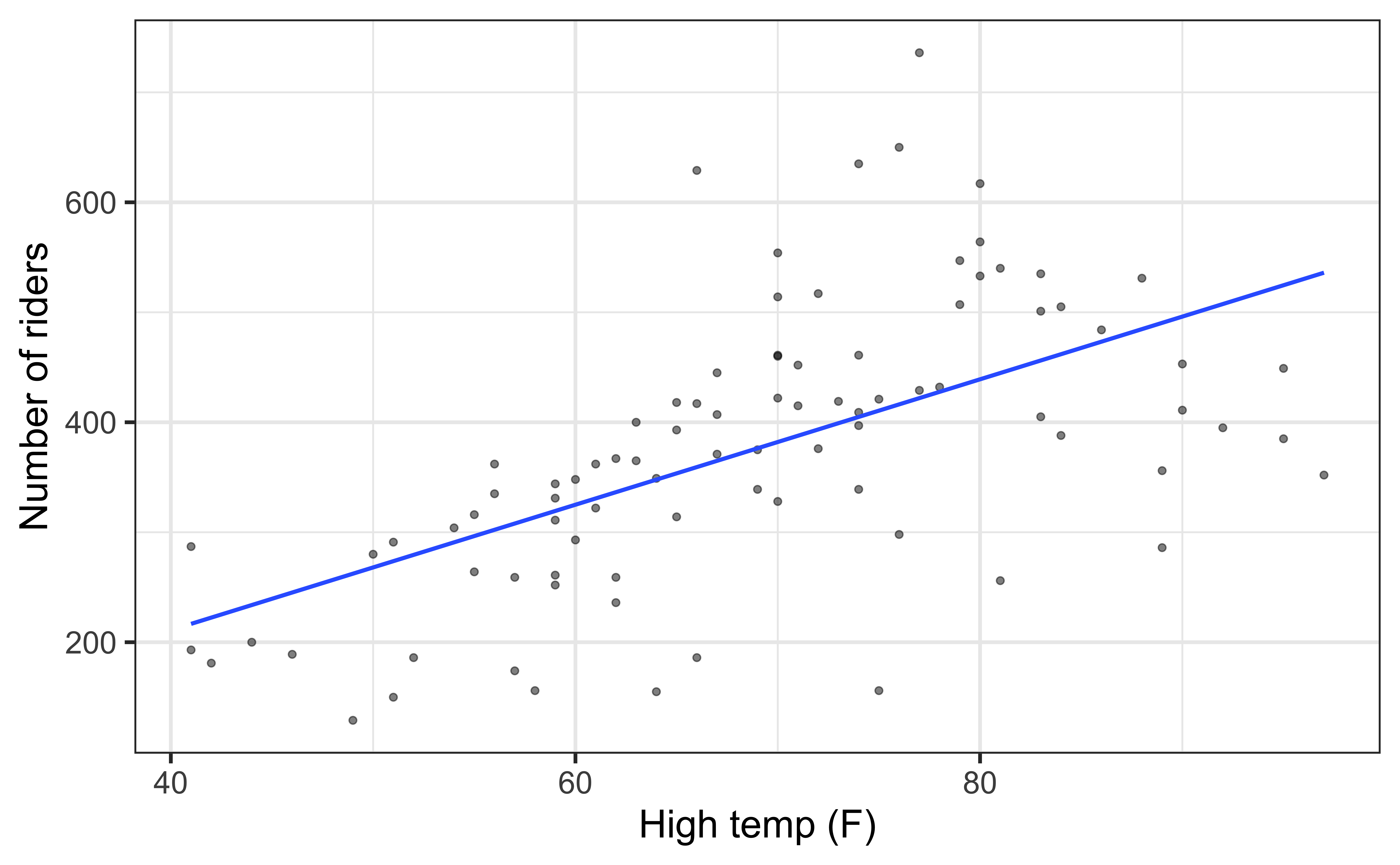
SLR model summary
SLR hypothesis test
| term | estimate | std.error | statistic | p.value |
|---|---|---|---|---|
| (Intercept) | -17.08 | 59.40 | -0.29 | 0.77 |
| hightemp | 5.70 | 0.85 | 6.72 | 0.00 |
- Set hypotheses: \(H_0: \beta_1 = 0\) vs. \(H_A: \beta_1 \ne 0\)
- Calculate test statistic and p-value: The test statistic is \(t= 6.72\) . The p-value is calculated using a \(t\) distribution with 88 degrees of freedom. The p-value is \(\approx 0\) .
- State the conclusion: The p-value is small, so we reject \(H_0\). The data provide strong evidence that high temperature is a helpful predictor for the number of daily riders, i.e. there is a linear relationship between high temperature and number of daily riders.
Multiple linear regression
rt_mlr_main_fit <- linear_reg() |>
  set_engine("lm") |>
  fit(volume ~ hightemp + season, data = rail_trail)

tidy(rt_mlr_main_fit) |> kable(digits = 2)| term | estimate | std.error | statistic | p.value |
|---|---|---|---|---|
| (Intercept) | -125.23 | 71.66 | -1.75 | 0.08 |
| hightemp | 7.54 | 1.17 | 6.43 | 0.00 |
| seasonSpring | 5.13 | 34.32 | 0.15 | 0.88 |
| seasonSummer | -76.84 | 47.71 | -1.61 | 0.11 |
Multiple linear regression
The multiple linear regression model assumes \[Y|X_1, X_2, \ldots, X_p \sim N(\beta_0 + \beta_1 X_1 + \beta_2 X_2 + \dots + \beta_p X_p, \sigma_\epsilon^2)\]
For a given observation \((x_{i1}, x_{i2}, \ldots, x_{ip}, y_i)\), we can rewrite the previous statement as
\[y_i = \beta_0 + \beta_1 x_{i1} + \beta_2 x_{i2} + \dots + \beta_p x_{ip} + \epsilon_{i} \hspace{10mm} \epsilon_i \sim N(0,\sigma_{\epsilon}^2)\]
Estimating \(\sigma_\epsilon\)
For a given observation \((x_{i1}, x_{i2}, \ldots,x_{ip}, y_i)\) the residual is \[e_i = y_{i} - (\hat{\beta}_0 + \hat{\beta}_1 x_{i1} + \hat{\beta}_{2} x_{i2} + \dots + \hat{\beta}_p x_{ip})\]
The estimated value of the regression standard error , \(\sigma_{\epsilon}\), is
\[\hat{\sigma}_\epsilon = \sqrt{\frac{\sum_{i=1}^ne_i^2}{n-p-1}}\]
As with SLR, we use \(\hat{\sigma}_{\epsilon}\) to calculate \(SE_{\hat{\beta}_j}\), the standard error of each coefficient. See Matrix Form of Linear Regression for more detail.
MLR hypothesis test: hightemp
- Set hypotheses: \(H_0: \beta_{hightemp} = 0\) vs. \(H_A: \beta_{hightemp} \ne 0\), given
seasonis in the model
- Calculate test statistic and p-value: The test statistic is \(t = 6.43\). The p-value is calculated using a \(t\) distribution with 86 \((n - p - 1)\) degrees of freedom. The p-value is \(\approx 0\).
- State the conclusion: The p-value is small, so we reject \(H_0\). The data provide strong evidence that high temperature for the day is a useful predictor in a model that already contains the season as a predictor for number of daily riders.
The model for season = Spring
| term | estimate | std.error | statistic | p.value |
|---|---|---|---|---|
| (Intercept) | -125.23 | 71.66 | -1.75 | 0.08 |
| hightemp | 7.54 | 1.17 | 6.43 | 0.00 |
| seasonSpring | 5.13 | 34.32 | 0.15 | 0.88 |
| seasonSummer | -76.84 | 47.71 | -1.61 | 0.11 |
\[ \begin{aligned} \widehat{volume} &= -125.23 + 7.54 \times \texttt{hightemp} + 5.13 \times \texttt{seasonSpring} - 76.84 \times \texttt{seasonSummer} \\ &= -125.23 + 7.54 \times \texttt{hightemp} + 5.13 \times 1 - 76.84 \times 0 \\ &= -120.10 + 7.54 \times \texttt{hightemp} \end{aligned} \]
The model for season = Summer
| term | estimate | std.error | statistic | p.value |
|---|---|---|---|---|
| (Intercept) | -125.23 | 71.66 | -1.75 | 0.08 |
| hightemp | 7.54 | 1.17 | 6.43 | 0.00 |
| seasonSpring | 5.13 | 34.32 | 0.15 | 0.88 |
| seasonSummer | -76.84 | 47.71 | -1.61 | 0.11 |
\[ \begin{aligned} \widehat{volume} &= -125.23 + 7.54 \times \texttt{hightemp} + 5.13 \times \texttt{seasonSpring} - 76.84 \times \texttt{seasonSummer} \\ &= -125.23 + 7.54 \times \texttt{hightemp} + 5.13 \times 0 - 76.84 \times 1 \\ &= -202.07 + 7.54 \times \texttt{hightemp} \end{aligned} \]
The model for season = Fall
| term | estimate | std.error | statistic | p.value |
|---|---|---|---|---|
| (Intercept) | -125.23 | 71.66 | -1.75 | 0.08 |
| hightemp | 7.54 | 1.17 | 6.43 | 0.00 |
| seasonSpring | 5.13 | 34.32 | 0.15 | 0.88 |
| seasonSummer | -76.84 | 47.71 | -1.61 | 0.11 |
\[ \begin{aligned} \widehat{volume} &= -125.23 + 7.54 \times \texttt{hightemp} + 5.13 \times \texttt{seasonSpring} - 76.84 \times \texttt{seasonSummer} \\ &= -125.23 + 7.54 \times \texttt{hightemp} + 5.13 \times 0 - 76.84 \times 0 \\ &= -125.23 + 7.54 \times \texttt{hightemp} \end{aligned} \]
The models
Same slope, different intercepts
season = Spring: \(-120.10 + 7.54 \times \texttt{hightemp}\)season = Summer: \(-202.07 + 7.54 \times \texttt{hightemp}\)season = Fall: \(-125.23 + 7.54 \times \texttt{hightemp}\)
Interaction terms
| term | estimate | std.error | statistic | p.value |
|---|---|---|---|---|
| (Intercept) | -10.53 | 166.80 | -0.06 | 0.95 |
| hightemp | 5.48 | 2.95 | 1.86 | 0.07 |
| seasonSpring | -293.95 | 190.33 | -1.54 | 0.13 |
| seasonSummer | 354.18 | 255.08 | 1.39 | 0.17 |
| hightemp:seasonSpring | 4.88 | 3.26 | 1.50 | 0.14 |
| hightemp:seasonSummer | -4.54 | 3.75 | -1.21 | 0.23 |
Do the data provide evidence of a significant interaction effect? Comment on the significance of the interaction terms.
Confidence interval for \(\beta_j\)
Confidence interval for \(\beta_j\)
The \(C\%\) confidence interval for \(\beta_j\) \[\hat{\beta}_j \pm t^* SE(\hat{\beta}_j)\] where \(t^*\) follows a \(t\) distribution with \(n - p - 1\) degrees of freedom.
Generically: We are \(C\%\) confident that the interval LB to UB contains the population coefficient of \(x_j\).
In context: We are \(C\%\) confident that for every one unit increase in \(x_j\), we expect \(y\) to change by LB to UB units, holding all else constant.
Confidence interval for \(\beta_j\)
| term | estimate | std.error | statistic | p.value | conf.low | conf.high |
|---|---|---|---|---|---|---|
| (Intercept) | -125.23 | 71.66 | -1.75 | 0.08 | -267.68 | 17.22 |
| hightemp | 7.54 | 1.17 | 6.43 | 0.00 | 5.21 | 9.87 |
| seasonSpring | 5.13 | 34.32 | 0.15 | 0.88 | -63.10 | 73.36 |
| seasonSummer | -76.84 | 47.71 | -1.61 | 0.11 | -171.68 | 18.00 |
CI for hightemp
| term | estimate | std.error | statistic | p.value | conf.low | conf.high |
|---|---|---|---|---|---|---|
| (Intercept) | -125.23 | 71.66 | -1.75 | 0.08 | -267.68 | 17.22 |
| hightemp | 7.54 | 1.17 | 6.43 | 0.00 | 5.21 | 9.87 |
| seasonSpring | 5.13 | 34.32 | 0.15 | 0.88 | -63.10 | 73.36 |
| seasonSummer | -76.84 | 47.71 | -1.61 | 0.11 | -171.68 | 18.00 |
We are 95% confident that for every degree Fahrenheit the day is warmer, the number of riders increases by 5.21 to 9.87, on average, holding season constant.
CI for seasonSpring
| term | estimate | std.error | statistic | p.value | conf.low | conf.high |
|---|---|---|---|---|---|---|
| (Intercept) | -125.23 | 71.66 | -1.75 | 0.08 | -267.68 | 17.22 |
| hightemp | 7.54 | 1.17 | 6.43 | 0.00 | 5.21 | 9.87 |
| seasonSpring | 5.13 | 34.32 | 0.15 | 0.88 | -63.10 | 73.36 |
| seasonSummer | -76.84 | 47.71 | -1.61 | 0.11 | -171.68 | 18.00 |
We are 95% confident that the number of riders on a Spring day is lower by 63.1 to higher by 73.4 compared to a Fall day, on average, holding high temperature for the day constant.
Is season a significant predictor of the number of riders, after accounting for high temperature?
Inference pitfalls
Large sample sizes
Caution
If the sample size is large enough, the test will likely result in rejecting \(H_0: \beta_j = 0\) even \(x_j\) has a very small effect on \(y\).
Consider the practical significance of the result not just the statistical significance.
Use the confidence interval to draw conclusions instead of relying only p-values.
Small sample sizes
Caution
If the sample size is small, there may not be enough evidence to reject \(H_0: \beta_j=0\).
When you fail to reject the null hypothesis, DON’T immediately conclude that the variable has no association with the response.
There may be a linear association that is just not strong enough to detect given your data, or there may be a non-linear association.
Conditions for inference
Full model
Including all available predictors
Fit:
Summarize:
# A tibble: 8 × 5
  term            estimate std.error statistic p.value
  <chr>              <dbl>     <dbl>     <dbl>   <dbl>
1 (Intercept)        17.6      76.6      0.230 0.819
2 hightemp            7.07      2.42     2.92  0.00450
3 avgtemp            -2.04      3.14    -0.648 0.519
4 seasonSpring       35.9      33.0      1.09  0.280
5 seasonSummer       24.2      52.8      0.457 0.649
6 cloudcover         -7.25      3.84    -1.89  0.0627
7 precip            -95.7      42.6     -2.25  0.0273
8 day_typeWeekend 35.9 22.4 1.60 0.113 Model conditions
Linearity: There is a linear relationship between the response and predictor variables.
Constant Variance: The variability about the least squares line is generally constant.
Normality: The distribution of the residuals is approximately normal.
Independence: The residuals are independent from each other.
Checking Linearity
Look at a plot of the residuals vs. predicted values
Look at a plot of the residuals vs. each predictor
Linearity is met if there is no discernible pattern in each of these plots
Residuals vs. predicted values

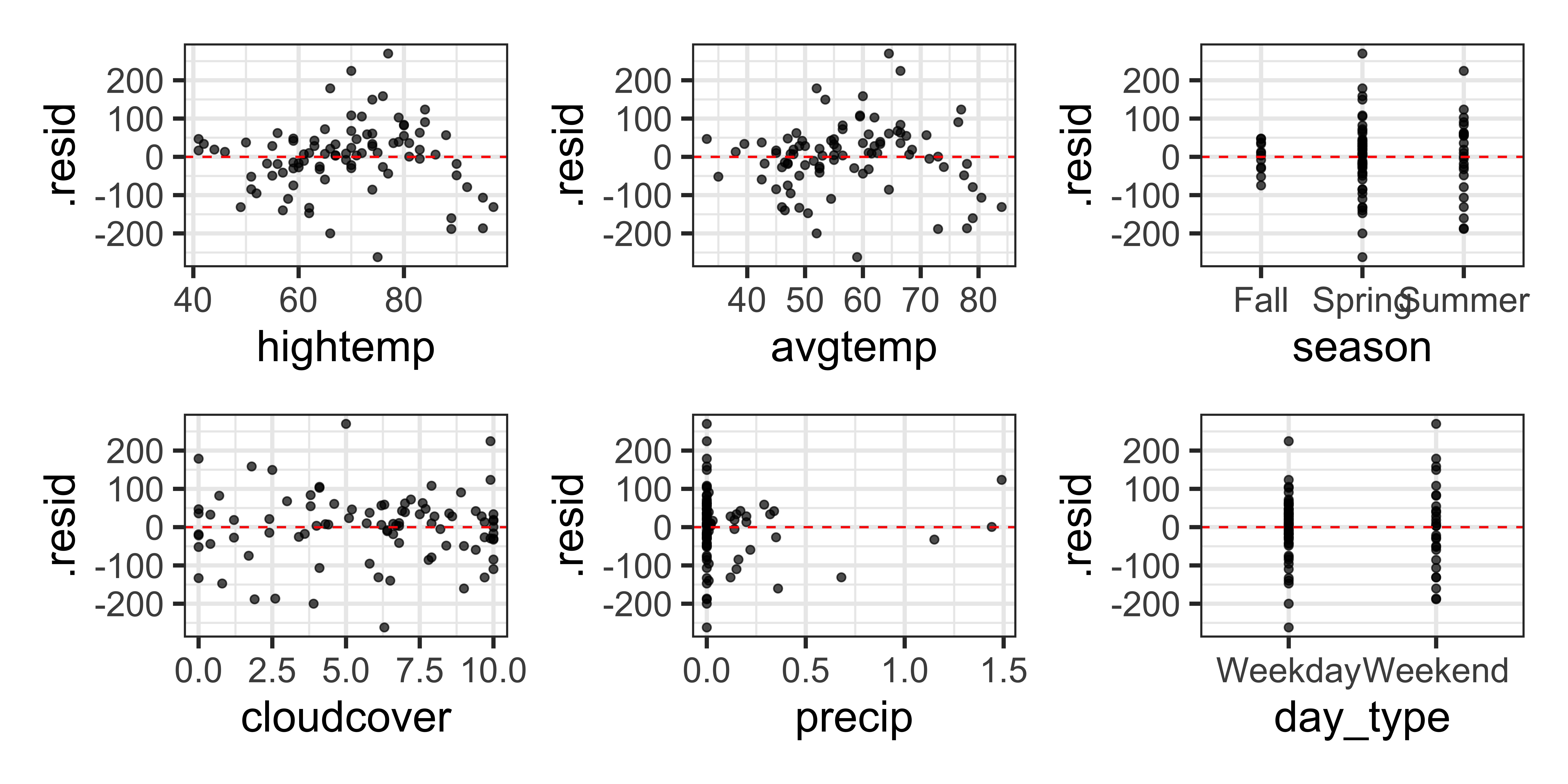
Residuals vs. each predictor
Checking linearity
The plot of the residuals vs. predicted values looked OK
The plots of residuals vs.
hightempandavgtempappear to have a parabolic pattern.The linearity condition does not appear to be satisfied given these plots.
Given this conclusion, what might be a next step in the analysis?
Checking constant variance
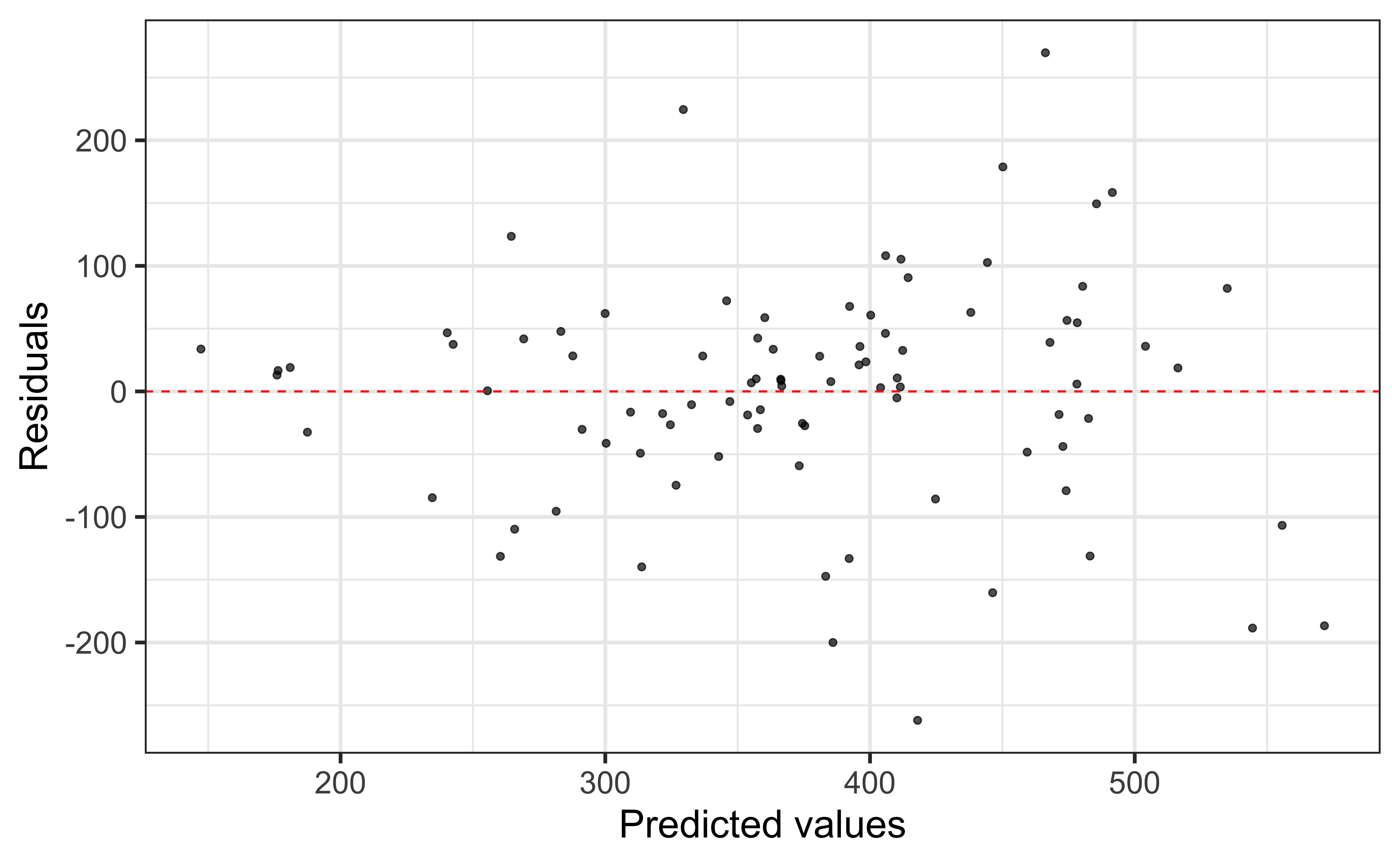
Does the constant variance condition appear to be satisfied?
Checking constant variance
The vertical spread of the residuals is not constant across the plot.
The constant variance condition is not satisfied.
We will talk about to address this later in the notes.
Checking normality
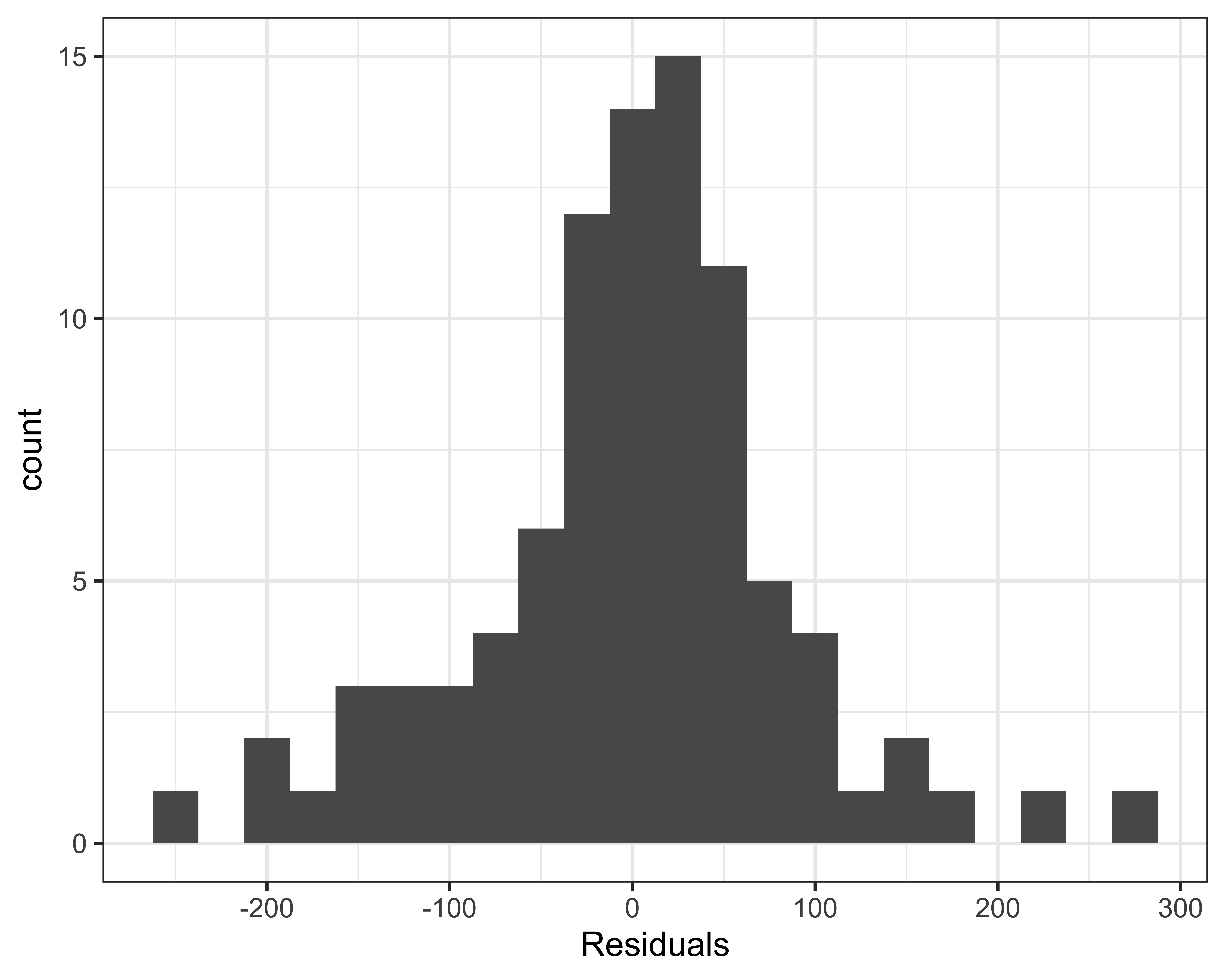
The distribution of the residuals is approximately unimodal and symmetric, so the normality condition is satisfied. The sample size 90 is sufficiently large to relax this condition if it was not satisfied.
Checking independence
We can often check the independence condition based on the context of the data and how the observations were collected.
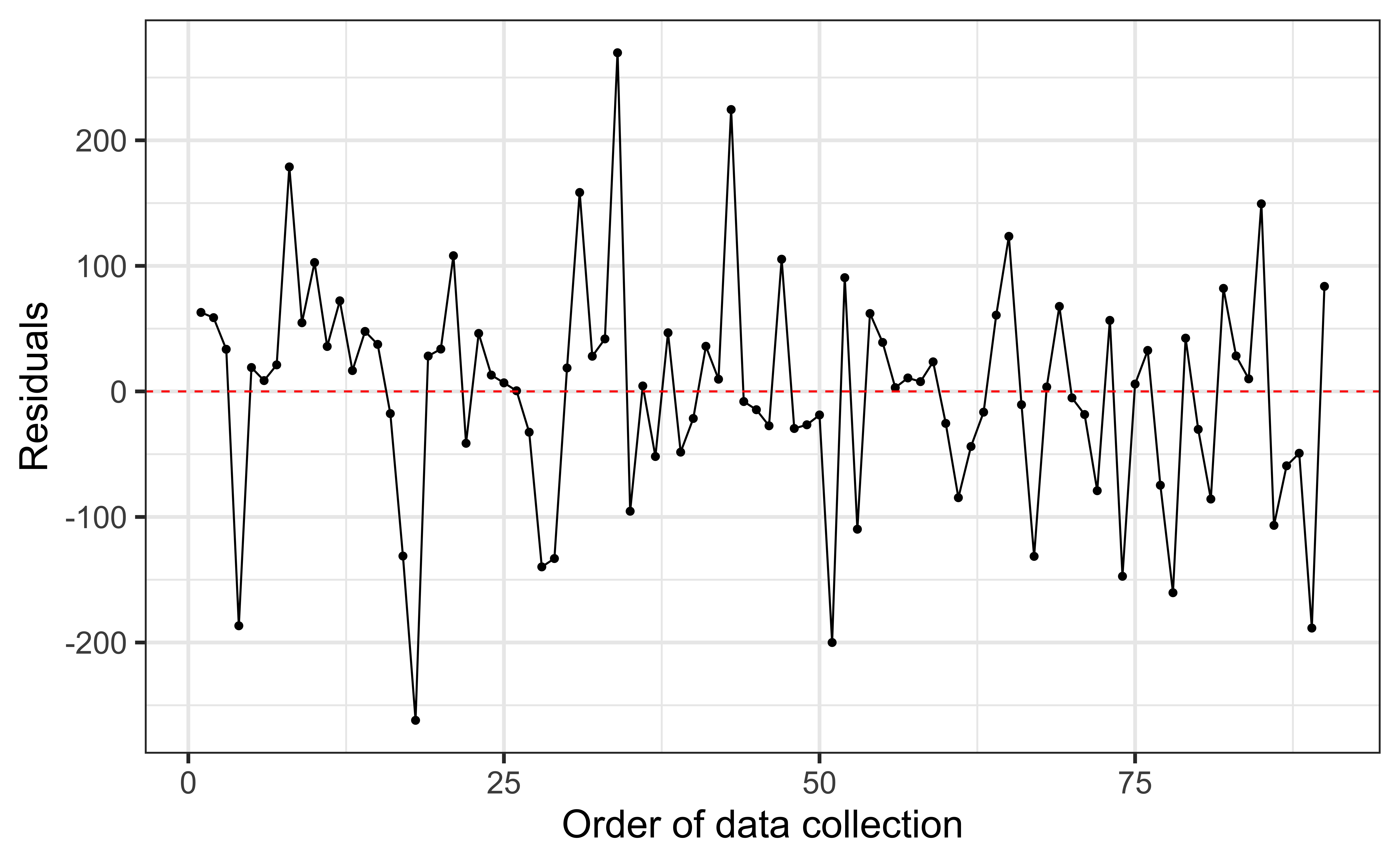
If the data were collected in a particular order, examine a scatterplot of the residuals versus order in which the data were collected.
If there is a grouping variable lurking in the background, check the residuals based on that grouping variable.
Checking independence
Residuals vs. order of data collection:
Checking independence
No clear pattern in the residuals vs. order of data collection plot.
Independence condition appears to be satisfied, as far as we can evaluate it.
Multicollinearity
What is multicollinearity
Multicollinearity is the case when two or more predictor variables are strongly correlated with one another
Example
Let’s assume the true population regression equation is \(y = 3 + 4x\)
Suppose we try estimating that equation using a model with variables \(x\) and \(z = x/10\)
\[ \begin{aligned}\hat{y}&= \hat{\beta}_0 + \hat{\beta}_1x + \hat{\beta}_2z\\ &= \hat{\beta}_0 + \hat{\beta}_1x + \hat{\beta}_2\frac{x}{10}\\ &= \hat{\beta}_0 + \bigg(\hat{\beta}_1 + \frac{\hat{\beta}_2}{10}\bigg)x \end{aligned} \]
Example
\[\hat{y} = \hat{\beta}_0 + \bigg(\hat{\beta}_1 + \frac{\hat{\beta}_2}{10}\bigg)x\]
We can set \(\hat{\beta}_1\) and \(\hat{\beta}_2\) to any two numbers such that \(\hat{\beta}_1 + \frac{\hat{\beta}_2}{10} = 4\)
Therefore, we are unable to choose the “best” combination of \(\hat{\beta}_1\) and \(\hat{\beta}_2\)
Why multicollinearity is a problem
When we have perfect collinearities, we are unable to get estimates for the coefficients
When we have almost perfect collinearities (i.e. highly correlated predictor variables), the standard errors for our regression coefficients inflate
In other words, we lose precision in our estimates of the regression coefficients
This impedes our ability to use the model for inference
It is also difficult to interpret the model coefficients
Detecting Multicollinearity
Multicollinearity may occur when…
- There are very high correlations \((r > 0.9)\) among two or more predictor variables, especially when the sample size is small
One (or more) predictor variables is an almost perfect linear combination of the others
There is a quadratic term in the model without mean-centering the variable first
There are interactions between two or more continuous variables
- Can reduce this by mean-centering the variables first
There is a categorical predictor with very few observations in the baseline level
Detecting multicollinearity in the EDA
- Look at a correlation matrix of the predictor variables, including all indicator variables
- Look out for values close to 1 or -1
- Look at a scatterplot matrix of the predictor variables
- Look out for plots that show a relatively linear relationship
- Look at the distribution of categorical predictors and avoid setting the baseline to a category with very few observations
Detecting Multicollinearity (VIF)
Variance Inflation Factor (VIF): Measure of multicollinearity in the regression model
\[VIF(\hat{\beta}_j) = \frac{1}{1-R^2_{X_j|X_{-j}}}\]
where \(R^2_{X_j|X_{-j}}\) is the proportion of variation \(X\) that is explained by the linear combination of the other explanatory variables in the model.
Detecting Multicollinearity (VIF)
Typically \(VIF > 10\) indicates concerning multicollinearity
Variables with similar values of VIF are typically the ones correlated with each other
Use the
vif()function in the rms R package to calculate VIF
VIF for rail trail model
       hightemp         avgtemp    seasonSpring    seasonSummer      cloudcover
      10.259978       13.086175        2.751577        5.841985        1.587485
         precip day_typeWeekend
       1.295352        1.125741
hightemp and avgtemp are correlated. We need to remove one of these variables and refit the model.
Model without hightemp
m1 <- linear_reg() |>
  set_engine("lm") |>
  fit(volume ~ . - hightemp, data = rail_trail)

m1 |>
  tidy() |>
kable(digits = 3)| term | estimate | std.error | statistic | p.value |
|---|---|---|---|---|
| (Intercept) | 76.071 | 77.204 | 0.985 | 0.327 |
| avgtemp | 6.003 | 1.583 | 3.792 | 0.000 |
| seasonSpring | 34.555 | 34.454 | 1.003 | 0.319 |
| seasonSummer | 13.531 | 55.024 | 0.246 | 0.806 |
| cloudcover | -12.807 | 3.488 | -3.672 | 0.000 |
| precip | -110.736 | 44.137 | -2.509 | 0.014 |
| day_typeWeekend | 48.420 | 22.993 | 2.106 | 0.038 |
Model without avgtemp
m2 <- linear_reg() |>
  set_engine("lm") |>
  fit(volume ~ . - avgtemp, data = rail_trail)

m2 |>
  tidy() |>
kable(digits = 3)| term | estimate | std.error | statistic | p.value |
|---|---|---|---|---|
| (Intercept) | 8.421 | 74.992 | 0.112 | 0.911 |
| hightemp | 5.696 | 1.164 | 4.895 | 0.000 |
| seasonSpring | 31.239 | 32.082 | 0.974 | 0.333 |
| seasonSummer | 9.424 | 47.504 | 0.198 | 0.843 |
| cloudcover | -8.353 | 3.435 | -2.431 | 0.017 |
| precip | -98.904 | 42.137 | -2.347 | 0.021 |
| day_typeWeekend | 37.062 | 22.280 | 1.663 | 0.100 |
Choosing a model
Model without hightemp:
| adj.r.squared | AIC | BIC |
|---|---|---|
| 0.42 | 1087.5 | 1107.5 |
Model without avgtemp:
| adj.r.squared | AIC | BIC |
|---|---|---|
| 0.47 | 1079.05 | 1099.05 |
Based on Adjusted \(R^2\), AIC, and BIC, the model without avgtemp is a better fit. Therefore, we choose to remove avgtemp from the model and leave hightemp in the model to deal with the multicollinearity.
Selected model (for now)
| term | estimate | std.error | statistic | p.value |
|---|---|---|---|---|
| (Intercept) | 8.421 | 74.992 | 0.112 | 0.911 |
| hightemp | 5.696 | 1.164 | 4.895 | 0.000 |
| seasonSpring | 31.239 | 32.082 | 0.974 | 0.333 |
| seasonSummer | 9.424 | 47.504 | 0.198 | 0.843 |
| cloudcover | -8.353 | 3.435 | -2.431 | 0.017 |
| precip | -98.904 | 42.137 | -2.347 | 0.021 |
| day_typeWeekend | 37.062 | 22.280 | 1.663 | 0.100 |
Variable transformations
Topics
Log transformation on the response variable
Log transformation on the predictor variable
Residuals vs. fitted for the selected model
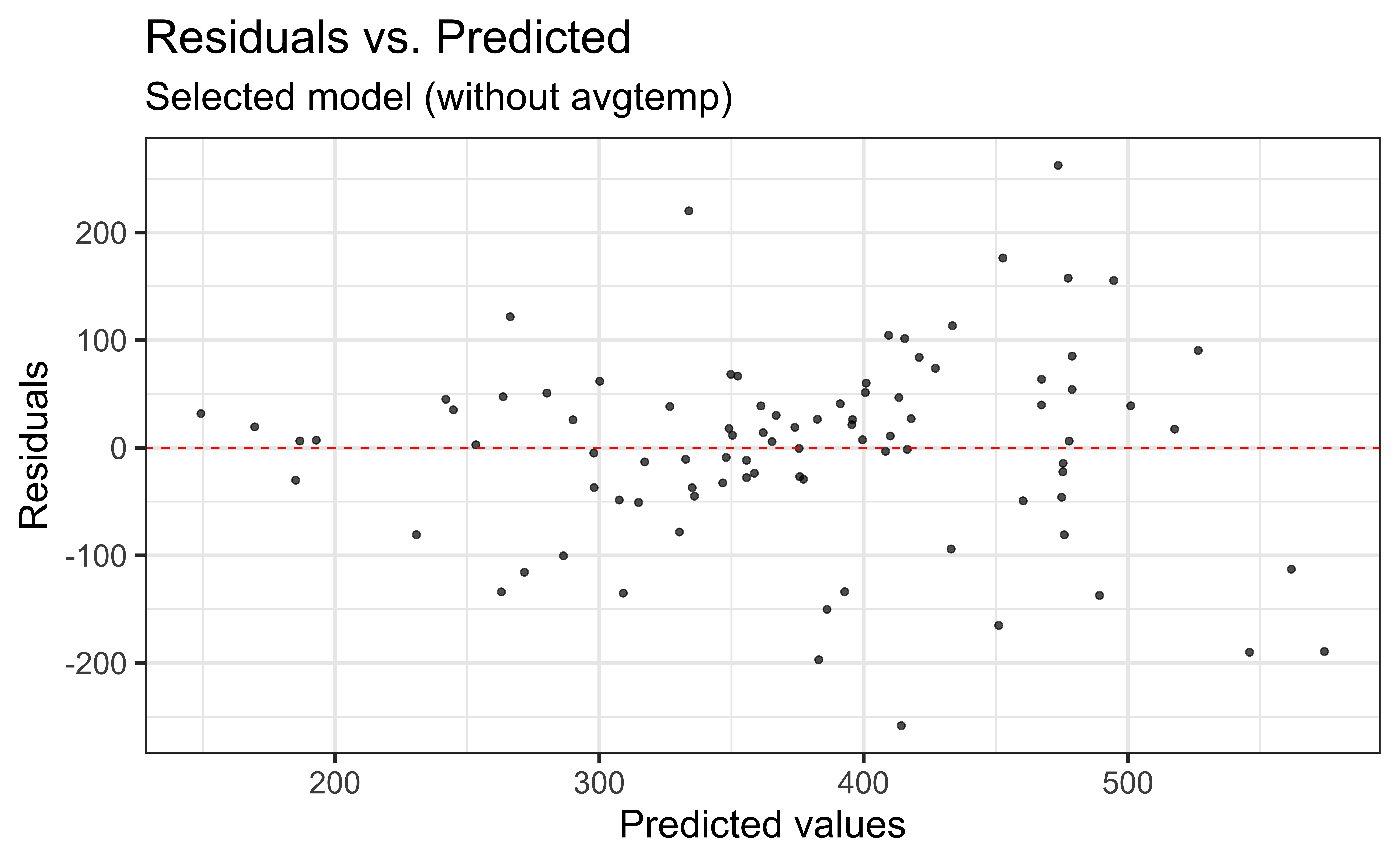
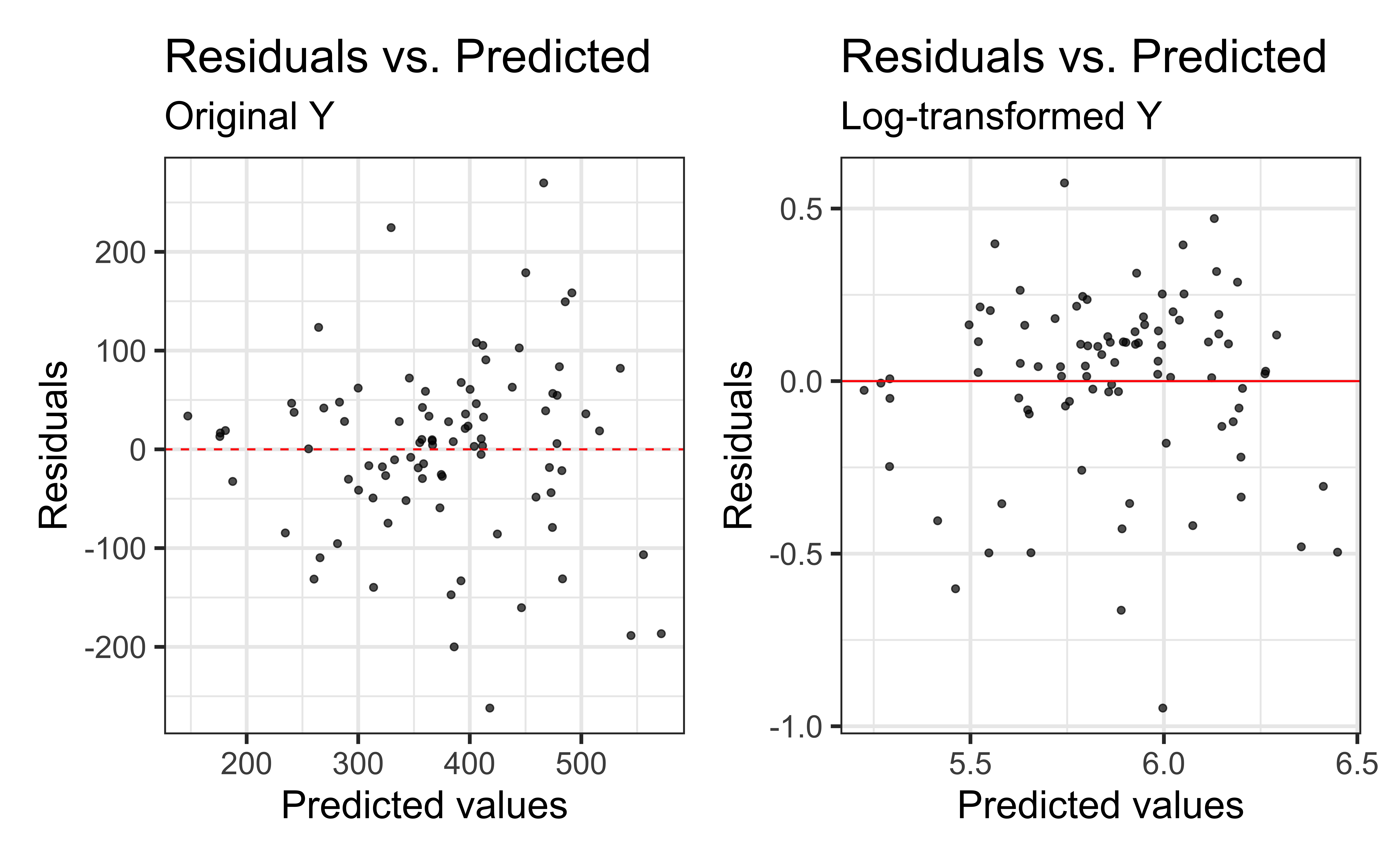
The constant variance condition is not satisfied. We can transform the response variable to address the violation in this condition.
Log transformation on the response variable
Identifying a need to transform \(Y\)
- Typically, a “fan-shaped” residual plot indicates the need for a transformation of the response variable \(Y\)
- There are multiple ways to transform a variable, e.g., \(\sqrt{Y}\), \(1/Y\), \(\log(Y)\)
- \(\log(Y)\) the most straightforward to interpret, so we use that transformation when possible
- When building a model:
- Choose a transformation and build the model on the transformed data
- Reassess the residual plots
- If the residuals plots did not sufficiently improve, try a new transformation!
Log transformation on \(Y\)
- If we apply a log transformation to the response variable, we want to estimate the parameters for the statistical model
\[ \log(Y) = \beta_0+ \beta_1 X_1 + \dots +\beta_pX_p + \epsilon, \hspace{10mm} \epsilon \sim N(0,\sigma^2_\epsilon) \]
- The regression equation is
\[\widehat{\log(Y)} = \hat{\beta}_0+ \hat{\beta}_1 X + \dots + \hat{\beta}_pX_p\]
Log transformation on \(Y\)
We want to interpret the model in terms of the original variable \(Y\), not \(\log(Y)\), so we need to write the regression equation in terms of \(Y\)
\[\begin{align}\hat{Y} &= \exp\{\hat{\beta}_0 + \hat{\beta}_1 X + \dots + \hat{\beta}_PX_P\}\\ &= \exp\{\hat{\beta}_0\}\exp\{\hat{\beta}_1X\}\dots\exp\{\hat{\beta}_pX_p\}\end{align}\]
Note
The predicted value \(\hat{Y}\) is the predicted median of \(Y\). Note, when the distribution of \(Y|X_1, \ldots, X_p\) is symmetric, then the median equals the mean. See the slides in the appendix for more detail.
Model interpretation
\[\begin{align}\hat{Y} &= \exp\{\hat{\beta}_0 + \hat{\beta}_1 X + \dots + \hat{\beta}_PX_P\}\\ &= \exp\{\hat{\beta}_0\}\exp\{\hat{\beta}_1X\}\dots\exp\{\hat{\beta}_pX_p\}\end{align}\]
Intercept: When \(X_1 = \dots = X_p =0\), \(Y\) is expected to be \(\exp\{\hat{\beta}_0\}\)
Slope: For every one unit increase in \(X_j\), the \(Y\) is expected to multiply by a factor of \(\exp\{\hat{\beta}_j\}\), holding all else constant
Why is the interpretation in terms of a multiplicative change?
Model for \(log(volume)\)
#fit model
log_rt_fit <- linear_reg() |>
  set_engine("lm") |>
  fit(log(volume) ~ hightemp + season + cloudcover + precip + day_type, data = rail_trail)

tidy(log_rt_fit) |>
kable(digits = 3)| term | estimate | std.error | statistic | p.value |
|---|---|---|---|---|
| (Intercept) | 4.738 | 0.219 | 21.667 | 0.000 |
| hightemp | 0.018 | 0.003 | 5.452 | 0.000 |
| seasonSpring | 0.026 | 0.094 | 0.283 | 0.778 |
| seasonSummer | -0.047 | 0.139 | -0.338 | 0.736 |
| cloudcover | -0.025 | 0.010 | -2.452 | 0.016 |
| precip | -0.294 | 0.123 | -2.397 | 0.019 |
| day_typeWeekend | 0.064 | 0.065 | 0.987 | 0.327 |
Interpretation of model for \(\log(volume)\)
| term | estimate | std.error | statistic | p.value |
|---|---|---|---|---|
| (Intercept) | 4.738 | 0.219 | 21.667 | 0.000 |
| hightemp | 0.018 | 0.003 | 5.452 | 0.000 |
| seasonSpring | 0.026 | 0.094 | 0.283 | 0.778 |
| seasonSummer | -0.047 | 0.139 | -0.338 | 0.736 |
| cloudcover | -0.025 | 0.010 | -2.452 | 0.016 |
| precip | -0.294 | 0.123 | -2.397 | 0.019 |
| day_typeWeekend | 0.064 | 0.065 | 0.987 | 0.327 |
Interpret the intercept in terms of (1)
log(volume)and (2)volume.Interpret the coefficient of
hightempin terms of (1)log(volume)and (2)volume.
Residuals for model with \(\log(volume)\)
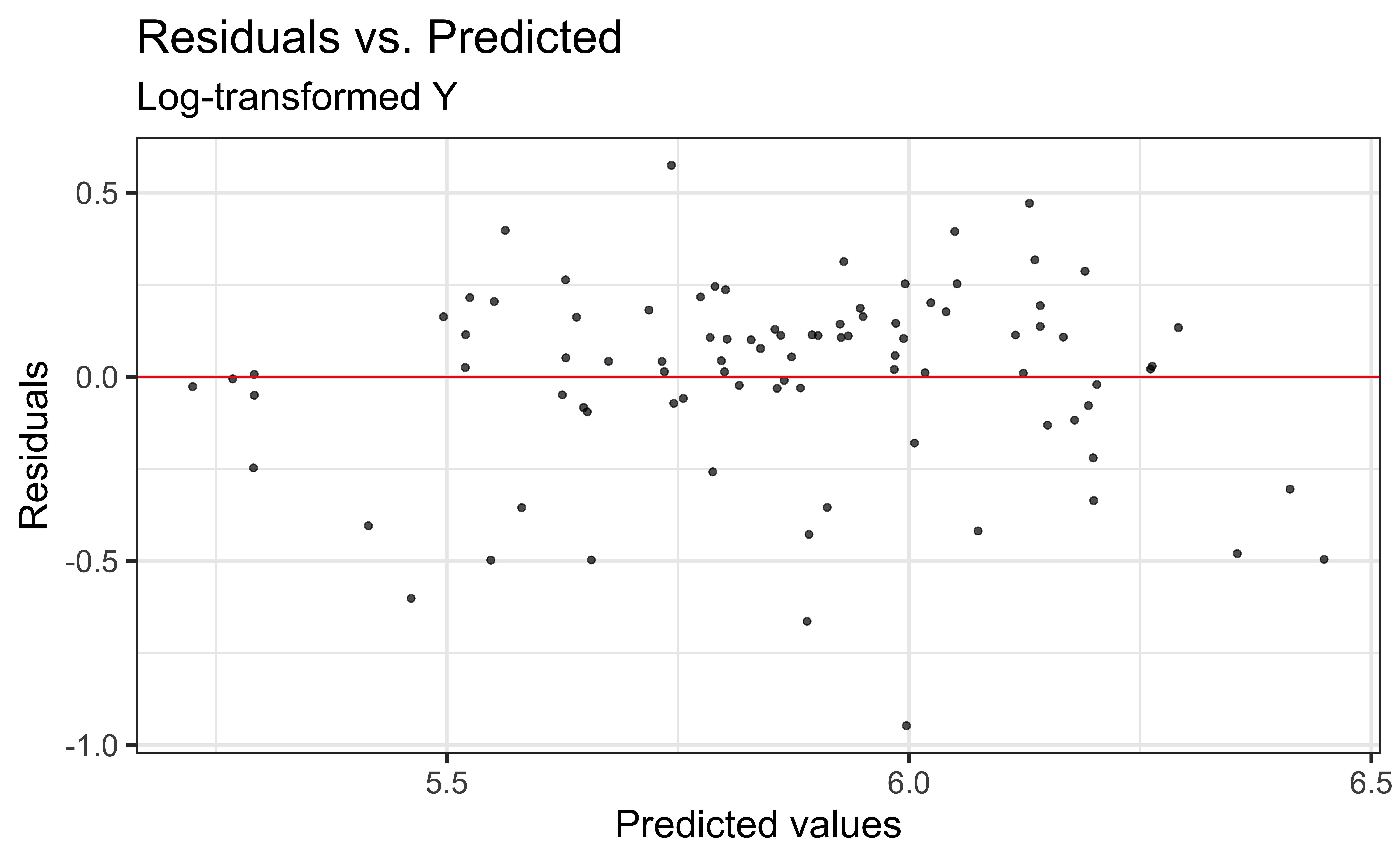
Compare residual plots
Log transformation on a predictor variable
Log Transformation on \(X\)
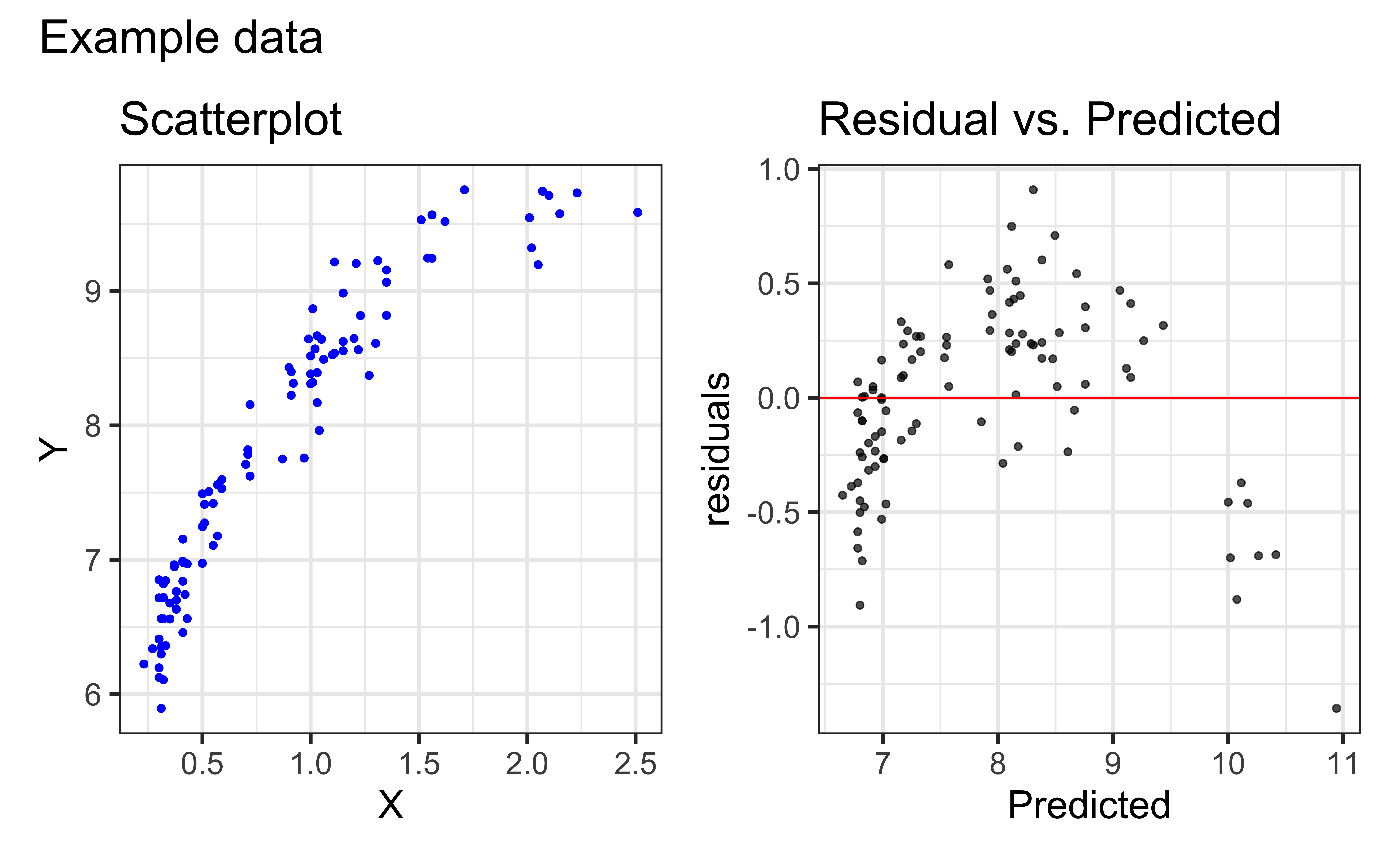
Try a transformation on \(X\) if the scatterplot shows some curvature but the variance is constant for all values of \(X\)
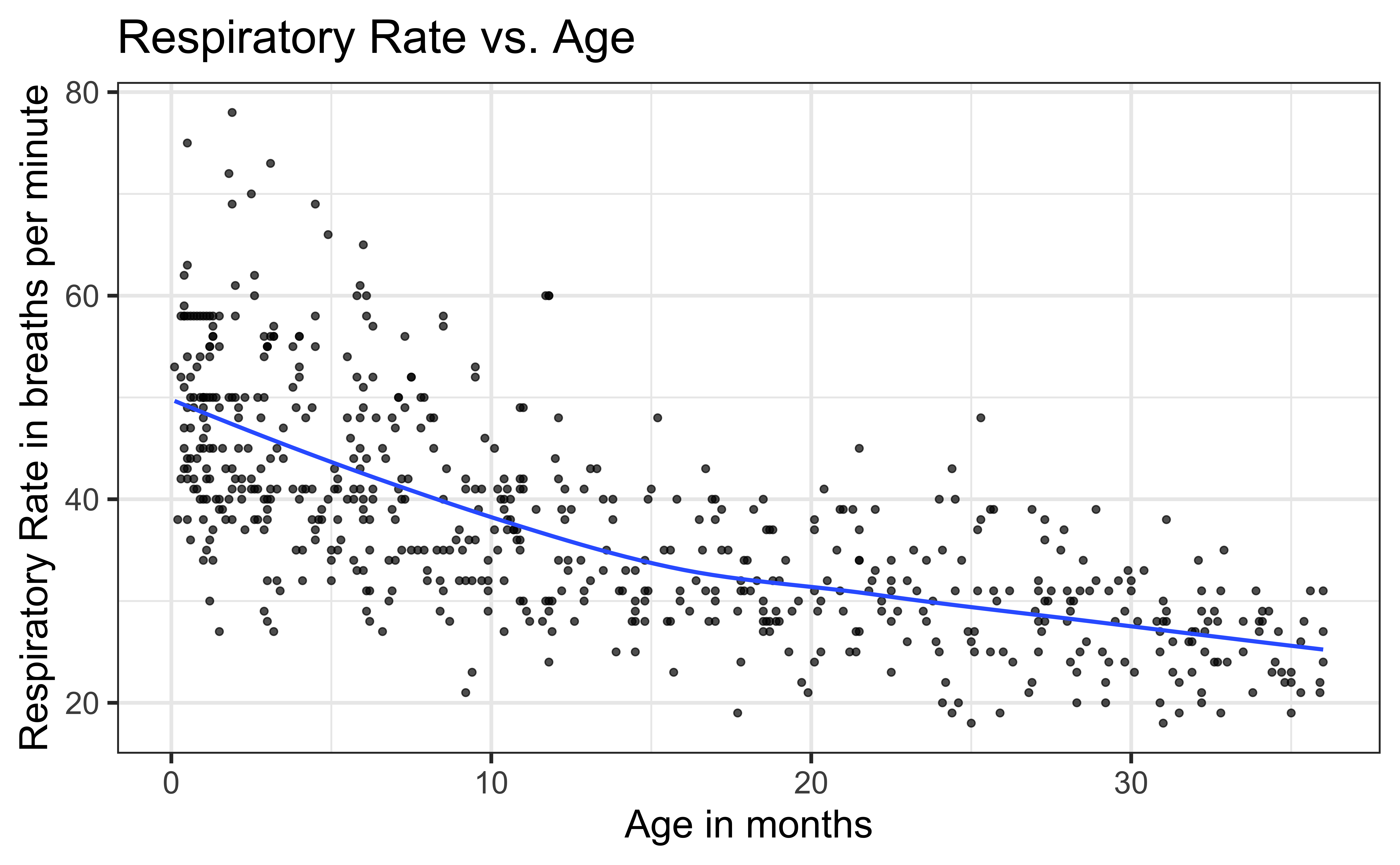
Respiratory Rate vs. Age
A high respiratory rate can potentially indicate a respiratory infection in children. In order to determine what indicates a “high” rate, we first want to understand the relationship between a child’s age and their respiratory rate.
The data contain the respiratory rate for 618 children ages 15 days to 3 years. It was obtained from the Sleuth3 R package and is originally form a 1994 publication “Reference Values for Respiratory Rate in the First 3 Years of Life”.
Variables:
Age: age in monthsRate: respiratory rate (breaths per minute)
Rate vs. Age
Model with Transformation on \(X\)
Suppose we have the following regression equation:
\[\hat{Y} = \hat{\beta}_0 + \hat{\beta}_1 \log(X)\]
Intercept: When \(X = 1\) \((\log(X) = 0)\), \(Y\) is expected to be \(\hat{\beta}_0\) (i.e. the mean of \(Y\) is \(\hat{\beta}_0\))
Slope: When \(X\) is multiplied by a factor of \(\mathbf{C}\), the mean of \(Y\) is expected to increase by \(\boldsymbol{\hat{\beta}_1}\mathbf{\log(C)}\) units
- Example: when \(X\) is multiplied by a factor of 2, \(Y\) is expected to increase by \(\boldsymbol{\hat{\beta}_1}\mathbf{\log(2)}\) units
Model interpretation
| term | estimate | std.error | statistic | p.value |
|---|---|---|---|---|
| (Intercept) | 50.135 | 0.632 | 79.330 | 0 |
| log(Age) | -5.982 | 0.263 | -22.781 | 0 |
\[\hat{\text{Rate}} = 50.135 - 5.982 \times \log\text{(Age)}\]
Interpret the intercept in the context of the data.
Interpret the slope in terms of age multiplying by 2 in the context of the data.
Learn more
See Log Transformations in Linear Regression for more details about interpreting regression models with log-transformed variables.
Appendix
Why \(Median(Y|X)\) instead of \(\mu_{Y|X}\)
Suppose we have a set of values
Note: \(\overline{\log(x)} \neq \log(\bar{x})\)
Why \(Median(Y|X)\) instead of \(\mu_{Y|X}\)
Note: \(\text{Median}(\log(x)) = \log(\text{Median}(x))\)
Mean, Median, and log
\[\overline{\log(x)} \neq \log(\bar{x})\]
Mean and median of \(\log(Y)\)
Recall that \(Y = \beta_0 + \beta_1 X\) is the mean value of the response at the given value of the predictor \(X\). This doesn’t hold when we log-transform the response variable.
Mathematically, the mean of the logged values is not necessarily equal to the log of the mean value. Therefore at a given value of \(X\)
\[ \begin{aligned}\exp\{\text{Mean}(\log(Y|X))\} \neq \text{Mean}(Y|X) \\[5pt] \Rightarrow \exp\{\beta_0 + \beta_1 X\} \neq \text{Mean}(Y|X) \end{aligned} \]
Mean and median of \(\log(y)\)
- However, the median of the logged values is equal to the log of the median value. Therefore,
\[\exp\{\text{Median}(\log(Y|X))\} = \text{Median}(Y|X)\]
- If the distribution of \(\log(Y)\) is symmetric about the regression line, for a given value \(X\), we can expect \(Mean(Y)\) and \(Median(Y)\) to be approximately equal.
