Model comparison + cross validation
Oct 18, 2023
Announcements
See Ed Discussion for upcoming events and internship opportunities
Statistics Experience due Mon, Nov 20 at 11:59pm
Please submit mid-semester feedback by Friday
Prof. Tackett office hours Fridays 1:30 - 3:30pm for the rest of the semester
Topics
- ANOVA for multiple linear regression and sum of squares
- Comparing models with \(R^2\) vs. \(R^2_{adj}\)
- Comparing models with AIC and BIC
- Occam’s razor and parsimony
- Cross validation
Computational setup
Introduction
Data: Restaurant tips
Which variables help us predict the amount customers tip at a restaurant?
# A tibble: 169 × 4
     Tip Party Meal   Age
   <dbl> <dbl> <chr>  <chr>
 1  2.99     1 Dinner Yadult
 2  2        1 Dinner Yadult
 3  5        1 Dinner SenCit
 4  4        3 Dinner Middle
 5 10.3      2 Dinner SenCit
 6  4.85     2 Dinner Middle
 7  5        4 Dinner Yadult
 8  4        3 Dinner Middle
 9  5        2 Dinner Middle
10  1.58     1 Dinner SenCit
# ℹ 159 more rows
Variables
Predictors:
Party: Number of people in the partyMeal: Time of day (Lunch, Dinner, Late Night)Age: Age category of person paying the bill (Yadult, Middle, SenCit)
Outcome: Tip: Amount of tip
Outcome: Tip
Predictors
Relevel categorical predictors
Predictors, again
Outcome vs. predictors
Fit and summarize model
tip_fit <- linear_reg() |>
  set_engine("lm") |>
  fit(Tip ~ Party + Age, data = tips)

tidy(tip_fit) |>
kable(digits = 3)| term | estimate | std.error | statistic | p.value |
|---|---|---|---|---|
| (Intercept) | -0.170 | 0.366 | -0.465 | 0.643 |
| Party | 1.837 | 0.124 | 14.758 | 0.000 |
| AgeMiddle | 1.009 | 0.408 | 2.475 | 0.014 |
| AgeSenCit | 1.388 | 0.485 | 2.862 | 0.005 |
Is this the best model to explain variation in tips?
Another model summary
Analysis of variance (ANOVA)
Analysis of variance (ANOVA)
ANOVA
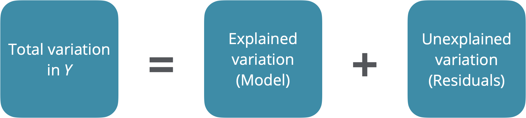
- Main Idea: Decompose the total variation on the outcome into:
the variation that can be explained by the each of the variables in the model
the variation that can’t be explained by the model (left in the residuals)
- If the variation that can be explained by the variables in the model is greater than the variation in the residuals, this signals that the model might be “valuable” (at least one of the \(\beta\)s not equal to 0)
ANOVA output in R1
ANOVA output, with totals
| term | df | sumsq | meansq | statistic | p.value |
|---|---|---|---|---|---|
| Party | 1 | 1188.64 | 1188.64 | 285.71 | 0 |
| Age | 2 | 38.03 | 19.01 | 4.57 | 0.01 |
| Residuals | 165 | 686.44 | 4.16 | ||
| Total | 168 | 1913.11 |
Sum of squares
| term | df | sumsq |
|---|---|---|
| Party | 1 | 1188.64 |
| Age | 2 | 38.03 |
| Residuals | 165 | 686.44 |
| Total | 168 | 1913.11 |
- \(SS_{Total}\): Total sum of squares, variability of outcome, \(\sum_{i = 1}^n (y_i - \bar{y})^2\)
- \(SS_{Error}\): Residual sum of squares, variability of residuals, \(\sum_{i = 1}^n (y_i - \hat{y}_i)^2\)
- \(SS_{Model} = SS_{Total} - SS_{Error}\): Variability explained by the model
Sum of squares: \(SS_{Total}\)
| term | df | sumsq |
|---|---|---|
| Party | 1 | 1188.64 |
| Age | 2 | 38.03 |
| Residuals | 165 | 686.44 |
| Total | 168 | 1913.11 |
\(SS_{Total}\): Total sum of squares, variability of outcome
\(\sum_{i = 1}^n (y_i - \bar{y})^2\) = 1913.11
Sum of squares: \(SS_{Error}\)
| term | df | sumsq |
|---|---|---|
| Party | 1 | 1188.64 |
| Age | 2 | 38.03 |
| Residuals | 165 | 686.44 |
| Total | 168 | 1913.11 |
\(SS_{Error}\): Residual sum of squares, variability of residuals
\(\sum_{i = 1}^n (y_i - \hat{y}_i)^2\) = 686.44
Sum of squares: \(SS_{Model}\)
| term | df | sumsq |
|---|---|---|
| Party | 1 | 1188.64 |
| Age | 2 | 38.03 |
| Residuals | 165 | 686.44 |
| Total | 168 | 1913.11 |
\(SS_{Model}\): Variability explained by the model
\(SS_{Total} - SS_{Error}\) = 1226.67
R-squared, \(R^2\)
Recall: \(R^2\) is the proportion of the variation in the response variable explained by the regression model.
\[ R^2 = \frac{SS_{Model}}{SS_{Total}} = 1 - \frac{SS_{Error}}{SS_{Total}} = 1 - \frac{686.44}{1913.11} = 0.641 \]
Model comparison
R-squared, \(R^2\)
- \(R^2\) will always increase as we add more variables to the model + If we add enough variables, we can always achieve \(R^2=100\%\)
- If we only use \(R^2\) to choose a best fit model, we will be prone to choose the model with the most predictor variables
Adjusted \(R^2\)
- Adjusted \(R^2\): measure that includes a penalty for unnecessary predictor variables
- Similar to \(R^2\), it is a measure of the amount of variation in the response that is explained by the regression model
- Differs from \(R^2\) by using the mean squares (sumsq/df) rather than sums of squares and therefore adjusting for the number of predictor variables
\(R^2\) and Adjusted \(R^2\)
\[R^2 = \frac{SS_{Model}}{SS_{Total}} = 1 - \frac{SS_{Error}}{SS_{Total}}\]
\[R^2_{adj} = 1 - \frac{SS_{Error}/(n-p-1)}{SS_{Total}/(n-1)}\]
where
\(n\) is the number of observations used to fit the model
\(p\) is the number of terms (not including the intercept) in the model
Using \(R^2\) and Adjusted \(R^2\)
- Adjusted \(R^2\) can be used as a quick assessment to compare the fit of multiple models; however, it should not be the only assessment!
- Use \(R^2\) when describing the relationship between the response and predictor variables
Comparing models with \(R^2_{adj}\)
- Why did we not use the full
recipe()workflow to fit Model 1 or Model 2? - Which model would we choose based on \(R^2\)?
- Which model would we choose based on Adjusted \(R^2\)?
- Which statistic should we use to choose the final model - \(R^2\) or Adjusted \(R^2\)? Why?
Vote on Ed Discussion [10:05am lecture][1:25pm lecture]
AIC & BIC
Estimators of prediction error and relative quality of models:
Akaike’s Information Criterion (AIC): \[AIC = n\log(SS_\text{Error}) - n \log(n) + 2(p+1)\]
Schwarz’s Bayesian Information Criterion (BIC): \[BIC = n\log(SS_\text{Error}) - n\log(n) + log(n)\times(p+1)\]
AIC & BIC
\[ \begin{aligned} & AIC = \color{blue}{n\log(SS_\text{Error})} - n \log(n) + 2(p+1) \\ & BIC = \color{blue}{n\log(SS_\text{Error})} - n\log(n) + \log(n)\times(p+1) \end{aligned} \]
First Term: Decreases as p increases
AIC & BIC
\[ \begin{aligned} & AIC = n\log(SS_\text{Error}) - \color{blue}{n \log(n)} + 2(p+1) \\ & BIC = n\log(SS_\text{Error}) - \color{blue}{n\log(n)} + \log(n)\times(p+1) \end{aligned} \]
Second Term: Fixed for a given sample size n
AIC & BIC
\[ \begin{aligned} & AIC = n\log(SS_\text{Error}) - n\log(n) + \color{blue}{2(p+1)} \\ & BIC = n\log(SS_\text{Error}) - n\log(n) + \color{blue}{\log(n)\times(p+1)} \end{aligned} \]
Third Term: Increases as p increases
Using AIC & BIC
\[ \begin{aligned} & AIC = n\log(SS_{Error}) - n \log(n) + \color{red}{2(p+1)} \\ & BIC = n\log(SS_{Error}) - n\log(n) + \color{red}{\log(n)\times(p+1)} \end{aligned} \]
Choose model with the smaller value of AIC or BIC
If \(n \geq 8\), the penalty for BIC is larger than that of AIC, so BIC tends to favor more parsimonious models (i.e. models with fewer terms)
Comparing models with AIC and BIC
Which model would we choose based on AIC?
Which model would we choose based on BIC?
Commonalities between criteria
- \(R^2_{adj}\), AIC, and BIC all apply a penalty for more predictors
- The penalty for added model complexity attempts to strike a balance between underfitting (too few predictors in the model) and overfitting (too many predictors in the model)
- Goal: Parsimony
Parsimony and Occam’s razor
The principle of parsimony is attributed to William of Occam (early 14th-century English nominalist philosopher), who insisted that, given a set of equally good explanations for a given phenomenon, the correct explanation is the simplest explanation1
Called Occam’s razor because he “shaved” his explanations down to the bare minimum
Parsimony in modeling:
- models should have as few parameters as possible
- linear models should be preferred to non-linear models
- experiments relying on few assumptions should be preferred to those relying on many
- models should be pared down until they are minimal adequate
- simple explanations should be preferred to complex explanations
In pursuit of Occam’s razor
Occam’s razor states that among competing hypotheses that predict equally well, the one with the fewest assumptions should be selected
Model selection follows this principle
We only want to add another variable to the model if the addition of that variable brings something valuable in terms of predictive power to the model
In other words, we prefer the simplest best model, i.e. parsimonious model
Alternate views
Sometimes a simple model will outperform a more complex model . . . Nevertheless, I believe that deliberately limiting the complexity of the model is not fruitful when the problem is evidently complex. Instead, if a simple model is found that outperforms some particular complex model, the appropriate response is to define a different complex model that captures whatever aspect of the problem led to the simple model performing well.
Radford Neal - Bayesian Learning for Neural Networks1
Other concerns with our approach
- All criteria we considered for model comparison require making predictions for our data and then uses the prediction error (\(SS_{Error}\)) somewhere in the formula
- But we’re making prediction for the data we used to build the model (estimate the coefficients), which can lead to overfitting
- Instead we should
split our data into testing and training sets
“train” the model on the training data and pick a few models we’re genuinely considering as potentially good models
test those models on the testing set
…and repeat this process multiple times
Cross validation
Spending our data
- We have already established that the idea of data spending where the test set was recommended for obtaining an unbiased estimate of performance.
- However, we usually need to understand the effectiveness of the model before using the test set.
- Typically we can’t decide on which final model to take to the test set without making model assessments.
- Remedy: Resampling to make model assessments on training data in a way that can generalize to new data.
Resampling for model assessment
Resampling is only conducted on the training set. The test set is not involved. For each iteration of resampling, the data are partitioned into two subsamples:
- The model is fit with the analysis set. Model fit statistics such as \(R^2_{Adj}\), AIC, and BIC are calculated based on this fit.
- The model is evaluated with the assessment set.
Resampling for model assessment

Image source: Kuhn and Silge. Tidy modeling with R.
Analysis and assessment sets
- Analysis set is analogous to training set.
- Assessment set is analogous to test set.
- The terms analysis and assessment avoids confusion with initial split of the data.
- These data sets are mutually exclusive.
Cross validation
More specifically, v-fold cross validation – commonly used resampling technique:
- Randomly split your training data into v partitions
- Use v-1 partitions for analysis, and the remaining 1 partition for analysis (model fit + model fit statistics)
- Repeat v times, updating which partition is used for assessment each time
Let’s give an example where v = 3…
To get started…
Split data into training and test sets
To get started…
Create recipe
To get started…
Specify model
Create workflow
══ Workflow ════════════════════════════════════════════════════════════════════
Preprocessor: Recipe
Model: linear_reg()

── Preprocessor ────────────────────────────────────────────────────────────────
0 Recipe Steps

── Model ───────────────────────────────────────────────────────────────────────
Linear Regression Model Specification (regression)

Computational engine: lm
Cross validation, step 1
Randomly split your training data into 3 partitions:

Tips: Split training data
Cross validation, steps 2 and 3
- Use v-1 partitions for analysis, and the remaining 1 partition for assessment
- Repeat v times, updating which partition is used for assessment each time

Tips: Fit resamples
# Resampling results
# 3-fold cross-validation
# A tibble: 3 × 4
  splits          id    .metrics         .notes
  <list>          <chr> <list>           <list>
1 <split [84/42]> Fold1 <tibble [2 × 4]> <tibble [0 × 3]>
2 <split [84/42]> Fold2 <tibble [2 × 4]> <tibble [0 × 3]>
3 <split [84/42]> Fold3 <tibble [2 × 4]> <tibble [0 × 3]>
Cross validation, now what?
- We’ve fit a bunch of models
- Now it’s time to use them to collect metrics (e.g., $R^2$, AIC, RMSE, etc. ) on each model and use them to evaluate model fit and how it varies across folds
Collect \(R^2\) and RMSE from CV
# A tibble: 2 × 6
  .metric .estimator  mean     n std_err .config
  <chr>   <chr>      <dbl> <int>   <dbl> <chr>
1 rmse    standard   2.10      3  0.243  Preprocessor1_Model1
2 rsq     standard   0.591     3  0.0728 Preprocessor1_Model1
Note: These are calculated using the assessment data
Deeper look into \(R^2\) and RMSE
# A tibble: 6 × 5
  id    .metric .estimator .estimate .config
  <chr> <chr>   <chr>          <dbl> <chr>
1 Fold1 rmse    standard       2.04  Preprocessor1_Model1
2 Fold1 rsq     standard       0.736 Preprocessor1_Model1
3 Fold2 rmse    standard       1.71  Preprocessor1_Model1
4 Fold2 rsq     standard       0.509 Preprocessor1_Model1
5 Fold3 rmse    standard       2.54  Preprocessor1_Model1
6 Fold3 rsq     standard       0.528 Preprocessor1_Model1
Better tabulation of \(R^2\) and RMSE from CV
How does RMSE compare to y?
Cross validation RMSE stats:
Calculate \(R^2_{Adj}\), AIC, and BIC for each fold
# Function to get Adj R-sq, AIC, BIC
calc_model_stats <- function(x) {
  glance(extract_fit_parsnip(x)) |>
    select(adj.r.squared, AIC, BIC)
}

# Fit model and calculate statistics for each fold
tips_fit_rs1 <-tips_wflow1 |>
  fit_resamples(resamples = folds,
                control = control_resamples(extract = calc_model_stats))

tips_fit_rs1
# Resampling results
# 3-fold cross-validation
# A tibble: 3 × 5
splits id .metrics .notes .extracts
<list> <chr> <list> <list> <list>
1 <split [84/42]> Fold1 <tibble [2 × 4]> <tibble [0 × 3]> <tibble [1 × 2]>
2 <split [84/42]> Fold2 <tibble [2 × 4]> <tibble [0 × 3]> <tibble [1 × 2]>
3 <split [84/42]> Fold3 <tibble [2 × 4]> <tibble [0 × 3]> <tibble [1 × 2]>Collect \(R^2_{Adj}\), AIC, BIC from CV
# A tibble: 3 × 4
  adj.r.squared   AIC   BIC Fold
          <dbl> <dbl> <dbl> <chr>
1         0.550  369.  386. Fold1
2         0.659  377.  394. Fold2
3         0.718  337.  354. Fold3
Note: These are based on the model fit from the analysis data
Cross validation in practice
To illustrate how CV works, we used
v = 3:- Analysis sets are 2/3 of the training set
- Each assessment set is a distinct 1/3
- The final resampling estimate of performance averages each of the 3 replicates
This was useful for illustrative purposes, but
v = 3is a poor choice in practiceValues of
vare most often 5 or 10; we generally prefer 10-fold cross-validation as a default
Recap
- ANOVA for multiple linear regression and sum of squares
- Comparing models with
- \(R^2\) vs. \(R^2_{Adj}\)
- AIC and BIC
- Occam’s razor and parsimony
Cross validation for
model evaluation
model comparison