# load packages
library(tidyverse)   # for data wrangling and visualization
library(tidymodels)  # for modeling
library(usdata)      # for the county_2019 dataset
library(openintro)   # for Duke Forest dataset
library(scales)      # for pretty axis labels
library(glue)        # for constructing character strings
library(knitr)       # for neatly formatted tables
library(kableExtra)  # also for neatly formatted tablesf


# set default theme and larger font size for ggplot2
ggplot2::theme_set(ggplot2::theme_bw(base_size = 16))SLR: Randomization test for the slope
Sep 13, 2022
Data: Duke Forest houses
Sampling is natural

- When you taste a spoonful of soup and decide the spoonful you tasted isn’t salty enough, that’s exploratory analysis
- If you generalize and conclude that your entire soup needs salt, that’s an inference
- For your inference to be valid, the spoonful you tasted (the sample) needs to be representative of the entire pot (the population)
Visualize the bootstrap distribution

Compute the CI
Permutation, visualized
- Each of the observed values for
area(and forprice) exist in both the observed data plot as well as the permutedpriceplot - The permutation removes the relationship between
areaandprice
`geom_smooth()` using formula = 'y ~ x'
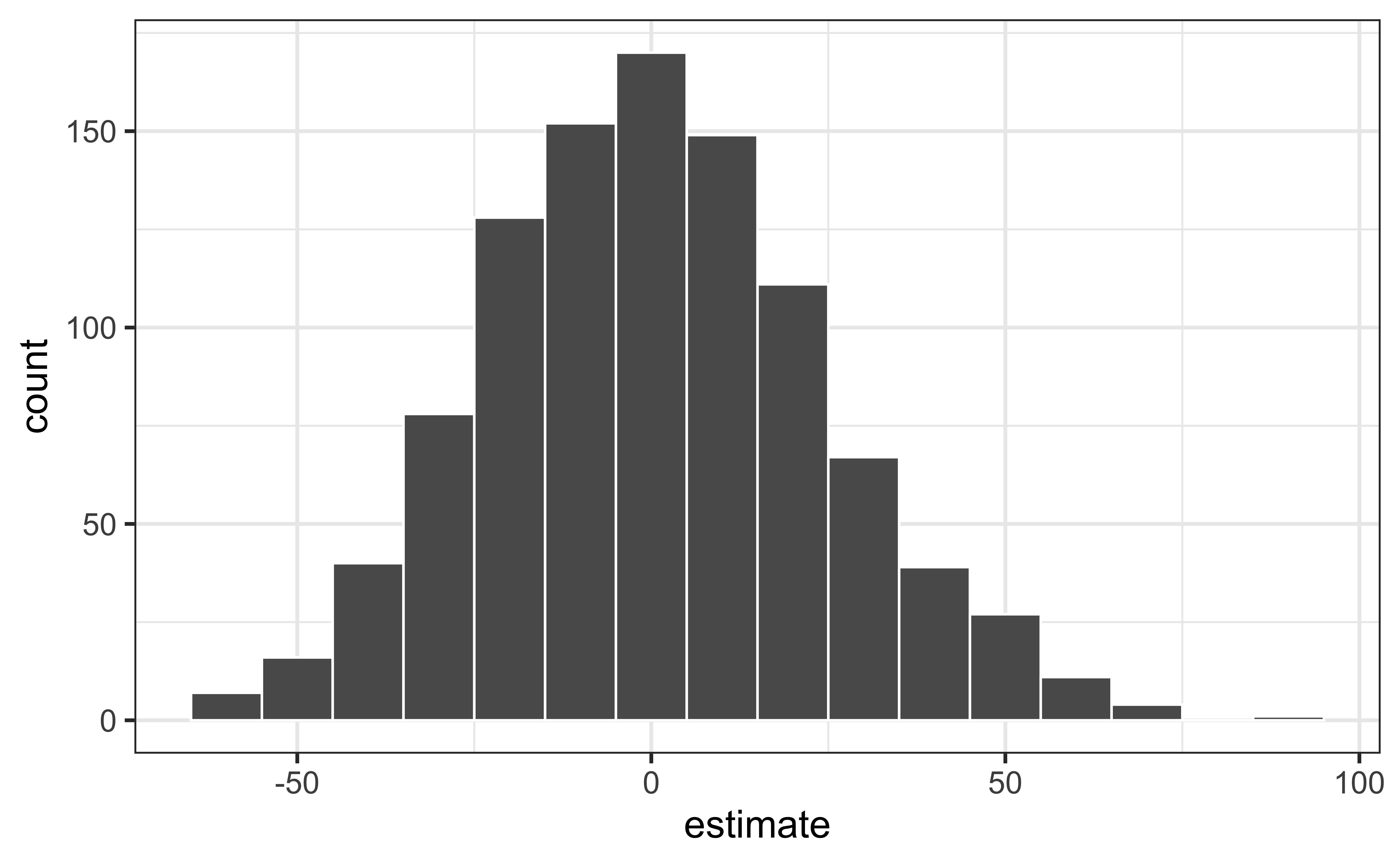
Permutation, repeated
Repeated permutations allow for quantifying the variability in the slope under the condition that there is no linear relationship (i.e., that the null hypothesis is true)
`geom_smooth()` using formula = 'y ~ x'
Concluding the hypothesis test
Is the observed slope of \(\hat{\beta_1} = 159\) (or an even more extreme slope) a likely outcome under the null hypothesis that \(\beta = 0\)? What does this mean for our original question: “Do the data provide sufficient evidence that \(\beta_1\) (the true slope for the population) is different from 0?”
Warning: Using `size` aesthetic for lines was deprecated in ggplot2 3.4.0.
ℹ Please use `linewidth` instead.
Warning: Removed 2 rows containing missing values (`geom_bar()`).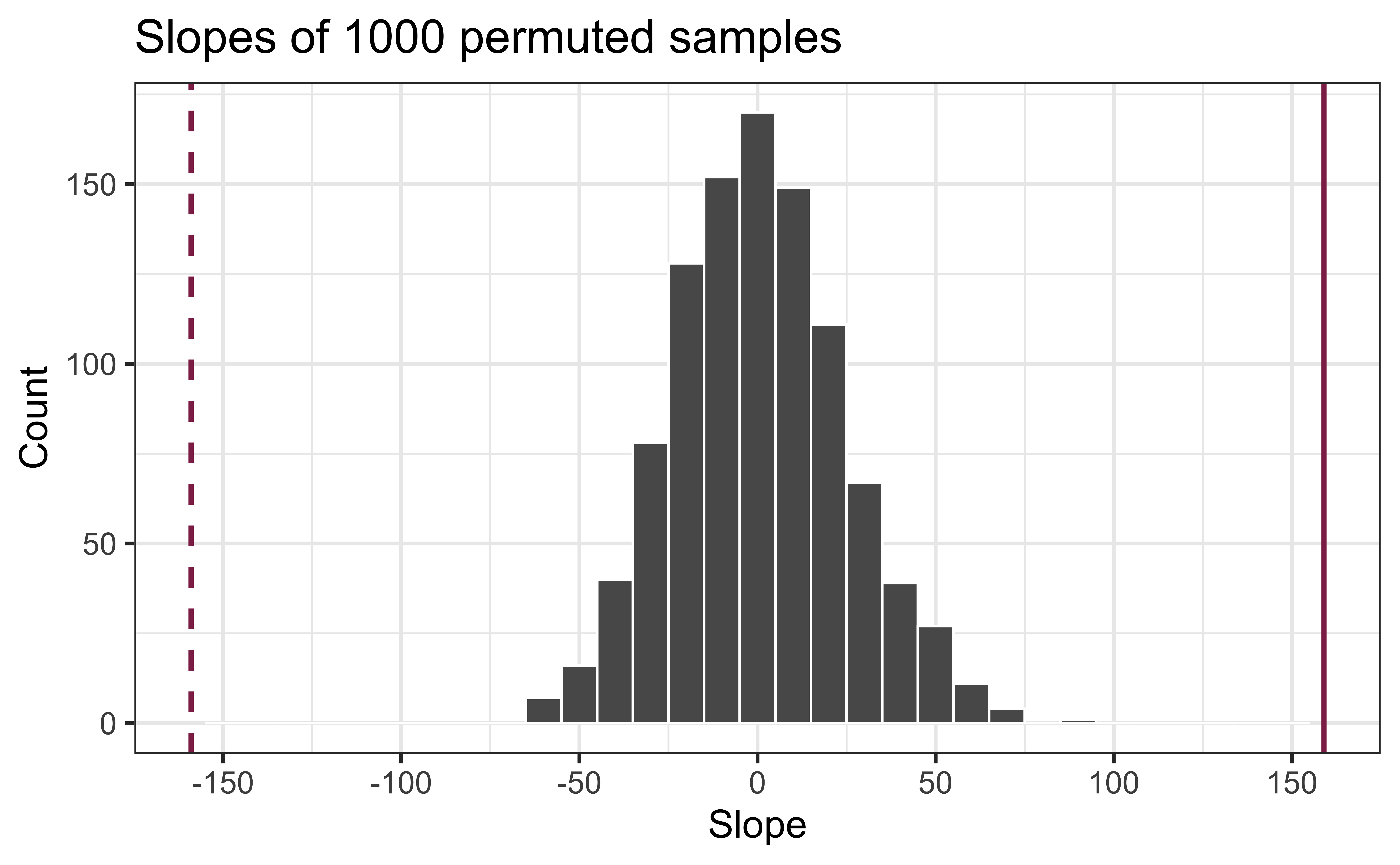
Visualize the null distribution
Reason around the p-value
In a world where the there is no relationship between the area of a Duke Forest house and in its price (\(\beta_1 = 0\)), what is the probability that we observe a sample of 98 houses where the slope fo the model predicting price from area is 159 or even more extreme?
Warning: Removed 2 rows containing missing values (`geom_bar()`).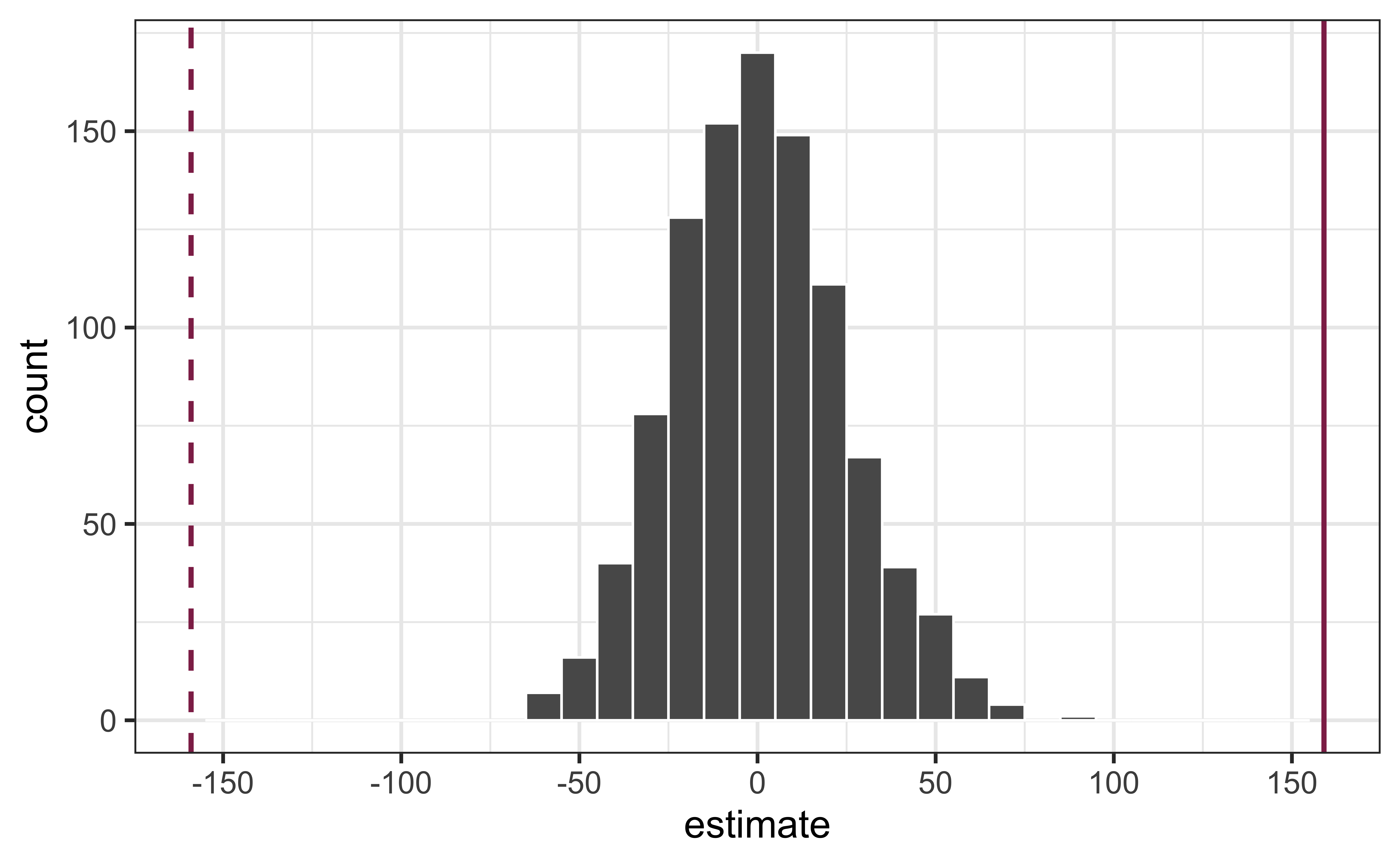
Mathematical representation, visualized
\[ Y|X \sim N(\beta_0 + \beta_1 X, \sigma_\epsilon^2) \]
`geom_smooth()` using formula = 'y ~ x'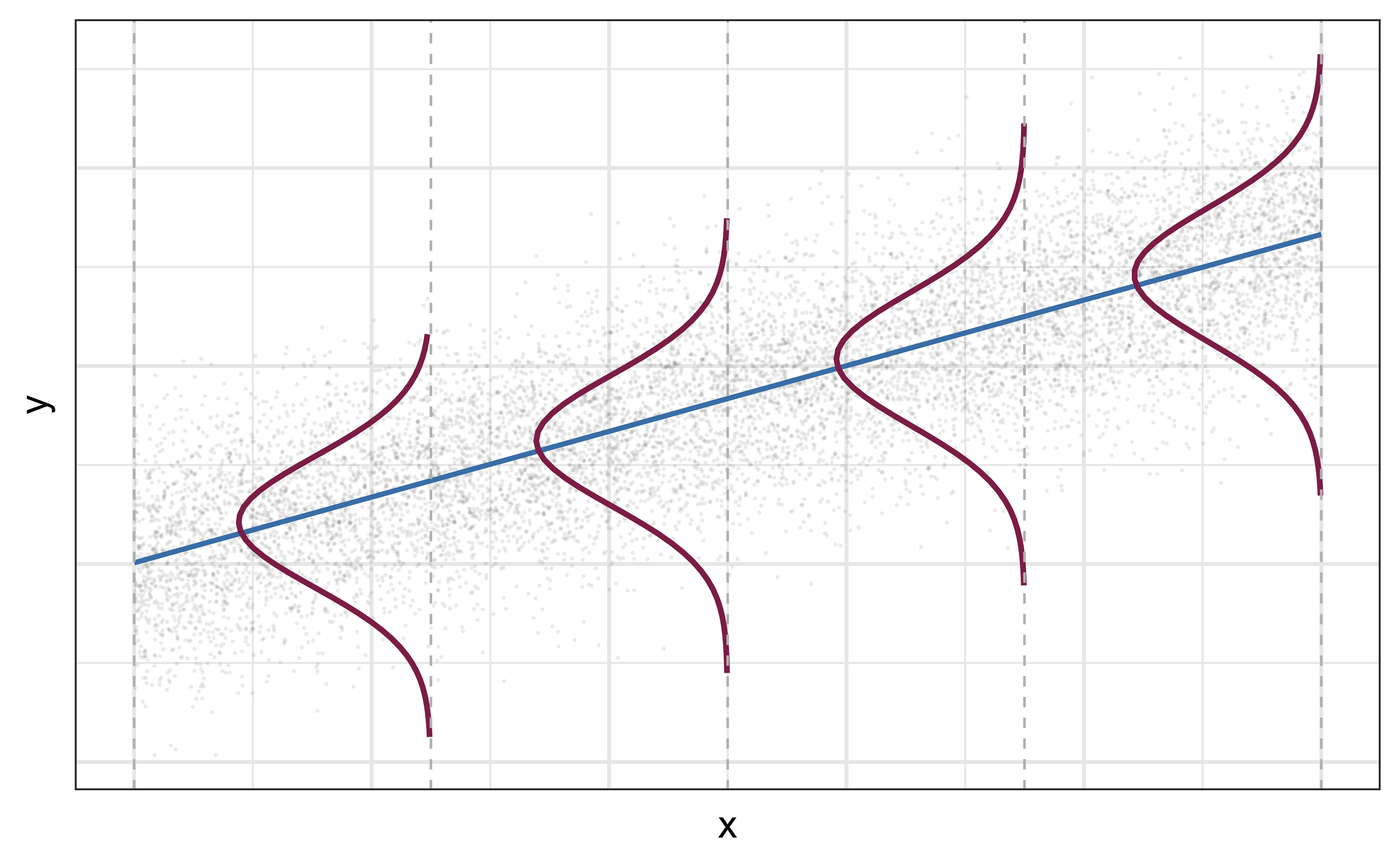
- Mean: \(\beta_0 + \beta_1 X\), the predicted value based on the regression model
- Variance: \(\sigma_\epsilon^2\), constant across the range of \(X\)
- How do we estimate \(\sigma_\epsilon^2\)?
Standard error of \(\hat{\beta}_1\)
\[ SE_{\hat{\beta}_1} = \hat{\sigma}_\epsilon\sqrt{\frac{1}{(n-1)s_X^2}} \]
or…
| term | estimate | std.error | statistic | p.value |
|---|---|---|---|---|
| (Intercept) | 116652.33 | 53302.46 | 2.19 | 0.03 |
| area | 159.48 | 18.17 | 8.78 | 0.00 |
![]()