“The Tulane Health Policy Case Competition gives teams of undergraduate students an opportunity to apply their talents and knowledge to put together a solution to a given health policy program Teams of up to three undergraduate students create policy-based solutions to a given problem. A workshop will be provided shortly after the case is released. Teams will construct PowerPoint presentations on solutions to the problem. Finalists will present to a panel of judges for real-time feedback.”
What: Each week, we will highlight a statisticians, data scientists, or other scholars from groups who have been historically marginalized in the field and whose work has made a significant impact.
Goal: Learn about scholars you may not see in traditional textbooks and see the breadth of past and current work in the field.
Participate: Present a Statistician of the Day or contribute to the CURV data base as your statistics experience
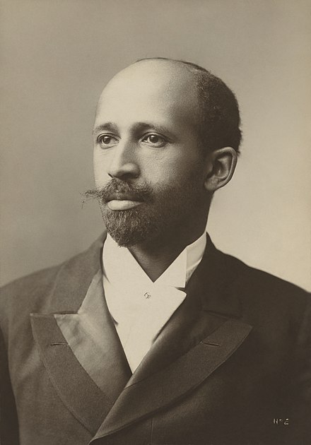
W.E.B. Du Bois
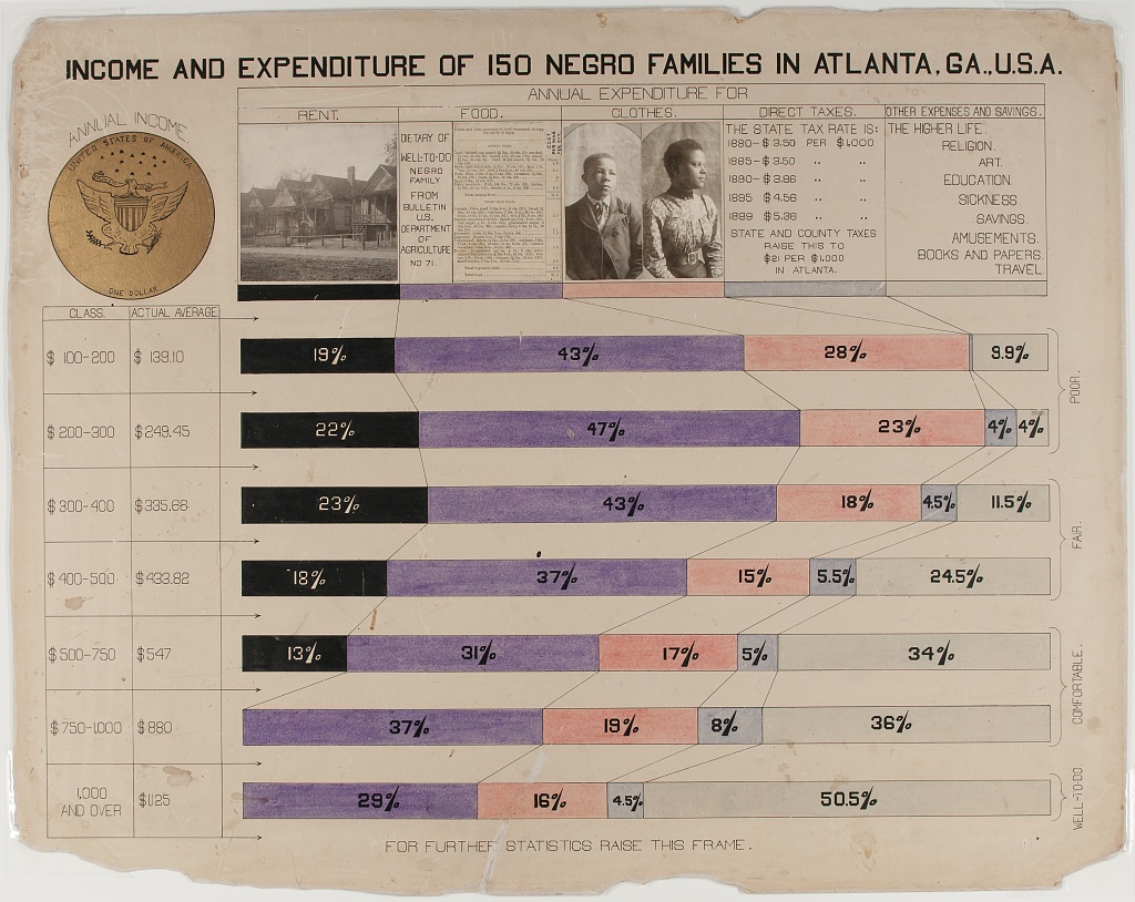
Du Bois (1868 - 1963) was a sociologist who contributed to the field of data visualization through infographics related to the African American in the early twentieth century.
In 1900 Du Bois contributed approximately 60 data visualizations to an exhibit at the Exposition Universelle in Paris, an exhibit designed to illustrate the progress made by African Americans since the end of slavery (only 37 years prior, in 1863).
The set of visualizations demonstrate how powerfully a picture can tell 1000 words, as the information Du Bois used was primarily available from public records (e.g., census and other government reports).
Why is there no error term in the regression equation?
Simulation-based inference
Bootstrap confidence intervals
Topics
Find range of plausible values for the slope using bootstrap confidence intervals
Computational setup
# load packageslibrary(tidyverse) # for data wrangling and visualizationlibrary(tidymodels) # for modelinglibrary(openintro) # for Duke Forest datasetlibrary(scales) # for pretty axis labelslibrary(glue) # for constructing character stringslibrary(knitr) # for neatly formatted tableslibrary(kableExtra) # also for neatly formatted tablesf# set default theme and larger font size for ggplot2ggplot2::theme_set(ggplot2::theme_bw(base_size =16))
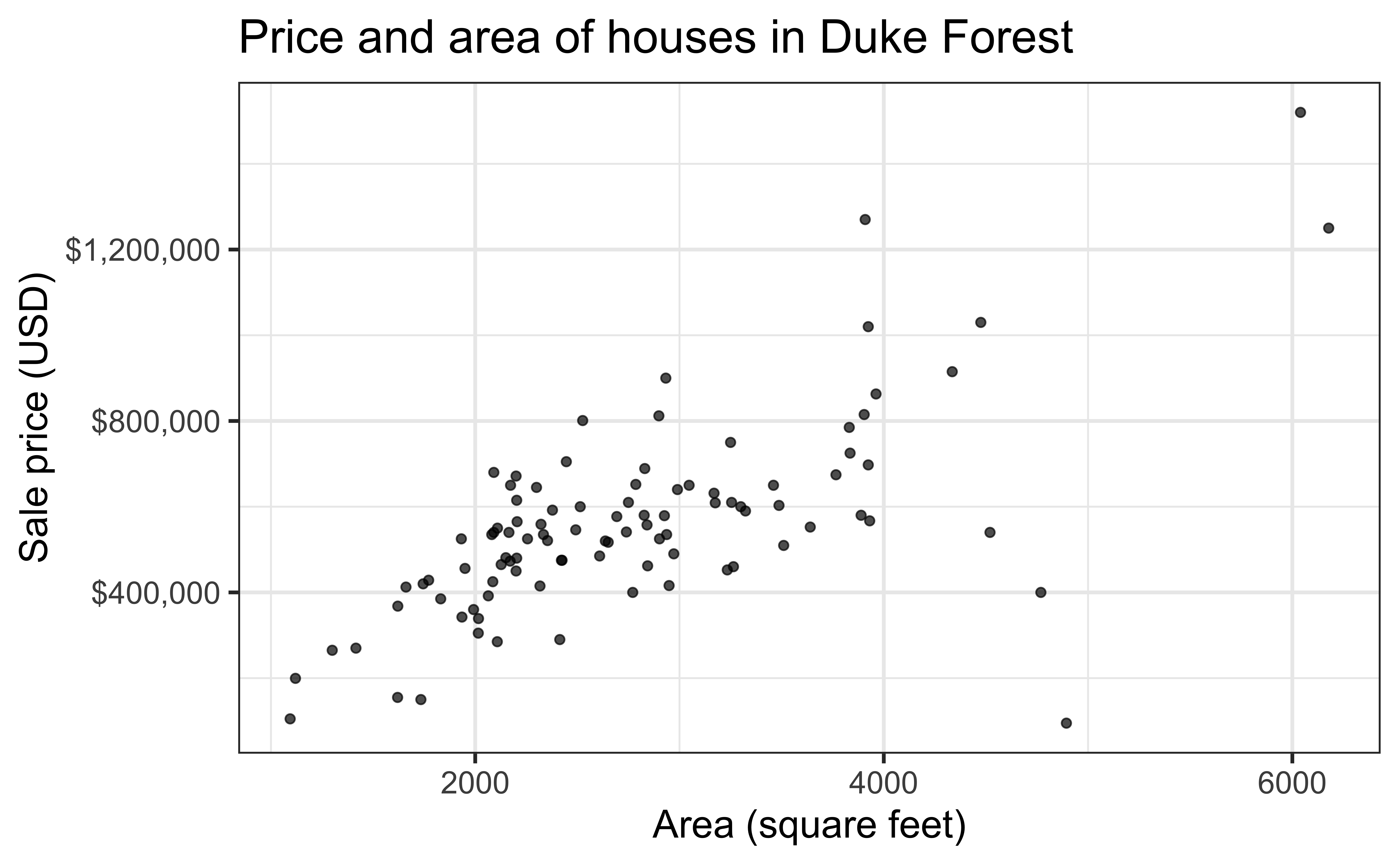
Data: Houses in Duke Forest
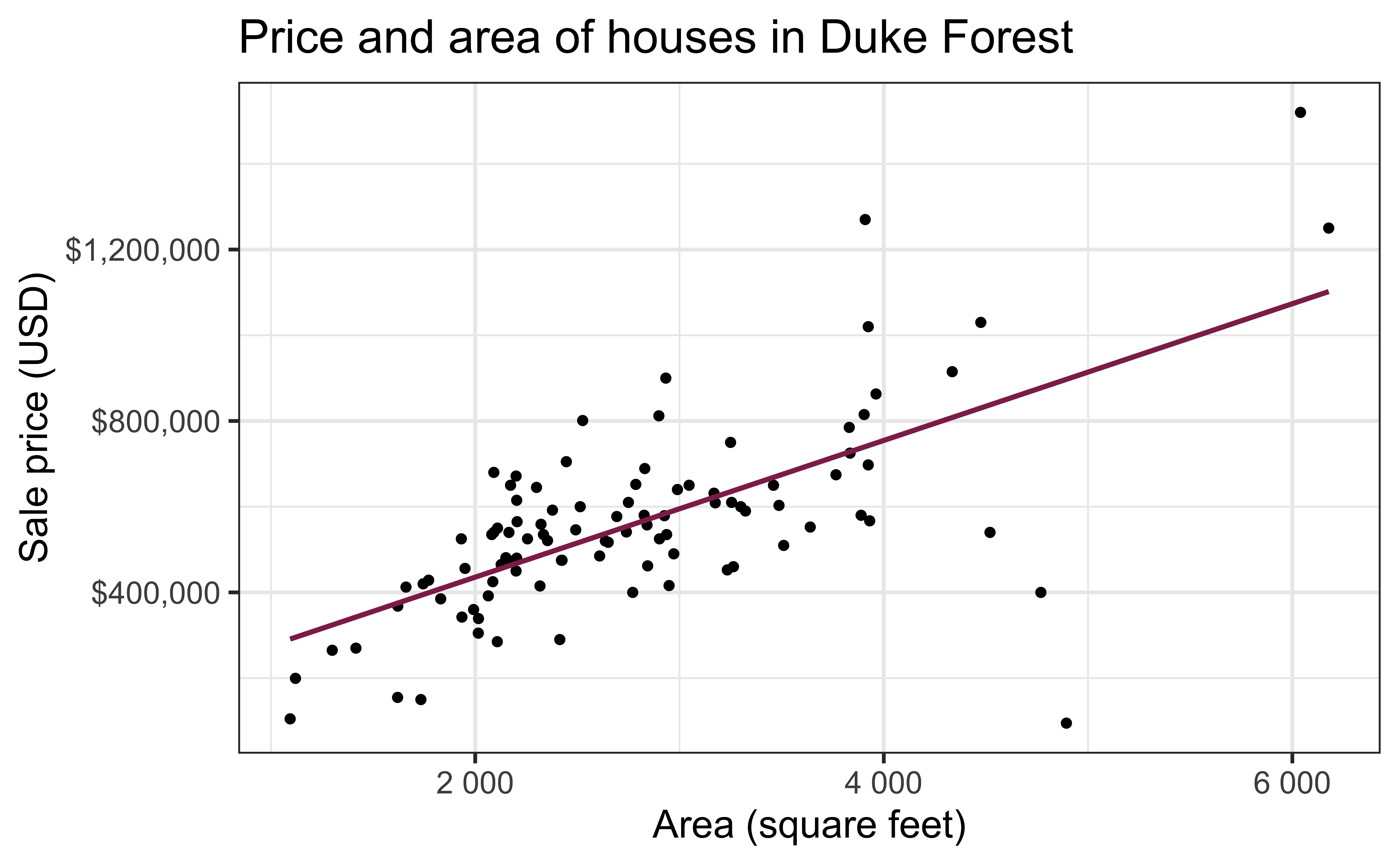
Data on houses that were sold in the Duke Forest neighborhood of Durham, NC around November 2020
Goal: Use the area (in square feet) to understand variability in the price of houses in Duke Forest.
Exploratory data analysis
Code
ggplot(duke_forest, aes(x = area, y = price)) +geom_point(alpha =0.7) +labs(x ="Area (square feet)",y ="Sale price (USD)",title ="Price and area of houses in Duke Forest" ) +scale_y_continuous(labels =label_dollar())
Modeling
df_fit <-linear_reg() |>#set_engine("lm") |>fit(price ~ area, data = duke_forest)tidy(df_fit) |>kable(digits =2) #neatly format table to 2 digits
term
estimate
std.error
statistic
p.value
(Intercept)
116652.33
53302.46
2.19
0.03
area
159.48
18.17
8.78
0.00
Intercept: Duke Forest houses that are 0 square feet are expected to sell, for $116,652, on average.
Is this interpretation useful?
Slope: For each additional square foot, we expect the sale price of Duke Forest houses to be higher by $159, on average.
From sample to population
For each additional square foot, we expect the sale price of Duke Forest houses to be higher by $159, on average.
This estimate is valid for the single sample of 98 houses.
But what if we’re not interested quantifying the relationship between the size and price of a house in this single sample?
What if we want to say something about the relationship between these variables for all houses in Duke Forest?
Statistical inference
Statistical inference provide methods and tools so we can use the single observed sample to make valid statements (inferences) about the population it comes from
For our inferences to be valid, the sample should be random and representative of the population we’re interested in
Inference for simple linear regression
Calculate a confidence interval for the slope, \(\beta_1\)
Conduct a hypothesis test for the slope,\(\beta_1\)
Confidence interval for the slope
Confidence interval
A plausible range of values for a population parameter is called a confidence interval
Using only a single point estimate is like fishing in a murky lake with a spear, and using a confidence interval is like fishing with a net
We can throw a spear where we saw a fish but we will probably miss, if we toss a net in that area, we have a good chance of catching the fish
Similarly, if we report a point estimate, we probably will not hit the exact population parameter, but if we report a range of plausible values we have a good shot at capturing the parameter
Confidence interval for the slope
A confidence interval will allow us to make a statement like “For each additional square foot, the model predicts the sale price of Duke Forest houses to be higher, on average, by $159, plus or minus X dollars.”
Should X be $10? $100? $1000?
If we were to take another sample of 98 would we expect the slope calculated based on that sample to be exactly $159? Off by $10? $100? $1000?
The answer depends on how variable (from one sample to another sample) the sample statistic (the slope) is
We need a way to quantify the variability of the sample statistic
Quantify the variability of the slope
for estimation
Two approaches:
Via simulation (what we’ll do today)
Via mathematical models (what we’ll do in the next class)
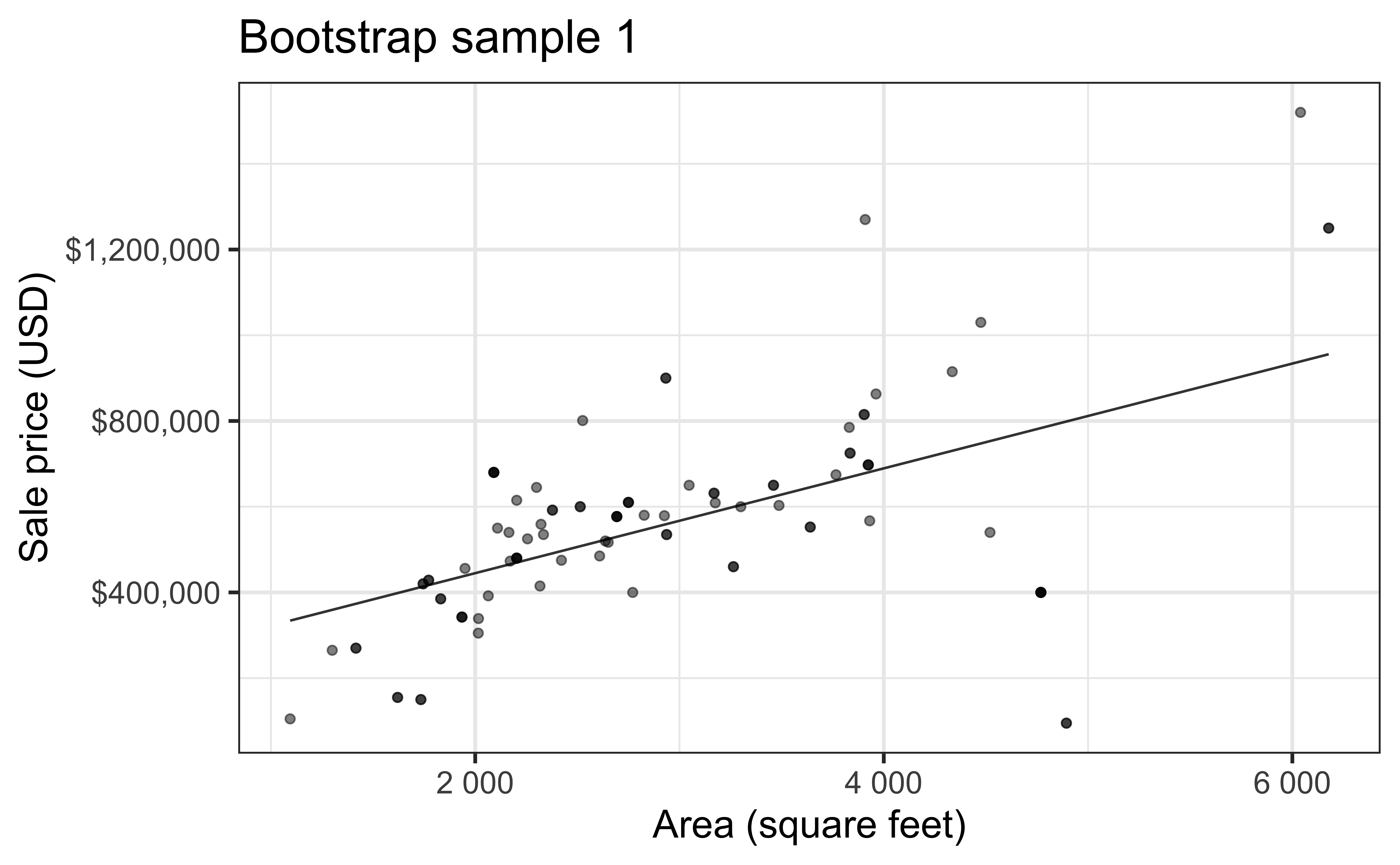
Bootstrapping to quantify the variability of the slope for the purpose of estimation:
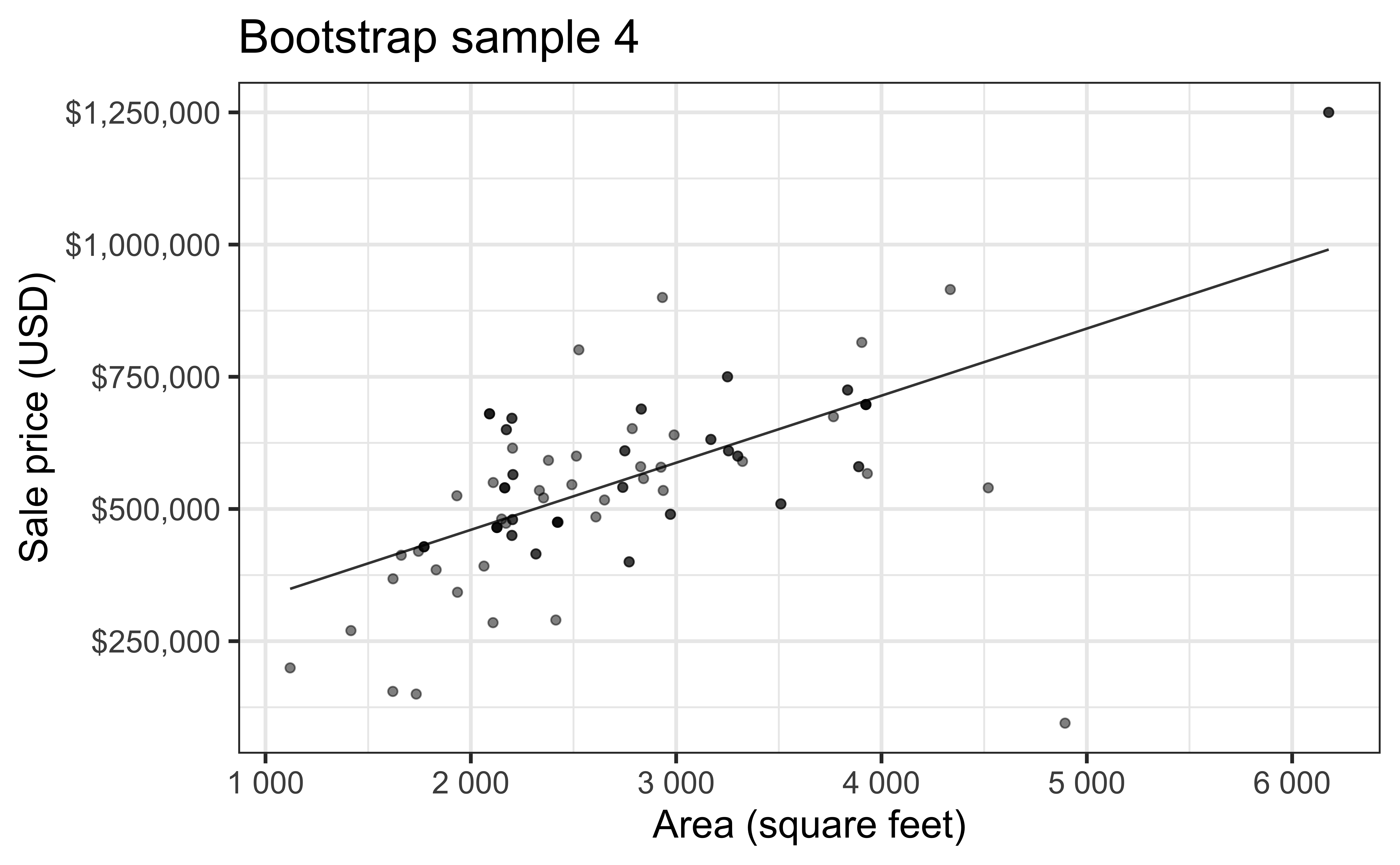
Bootstrap new samples from the original sample
Fit models to each of the samples and estimate the slope
Use features of the distribution of the bootstrapped slopes to construct a confidence interval
Bootstrap sample 1
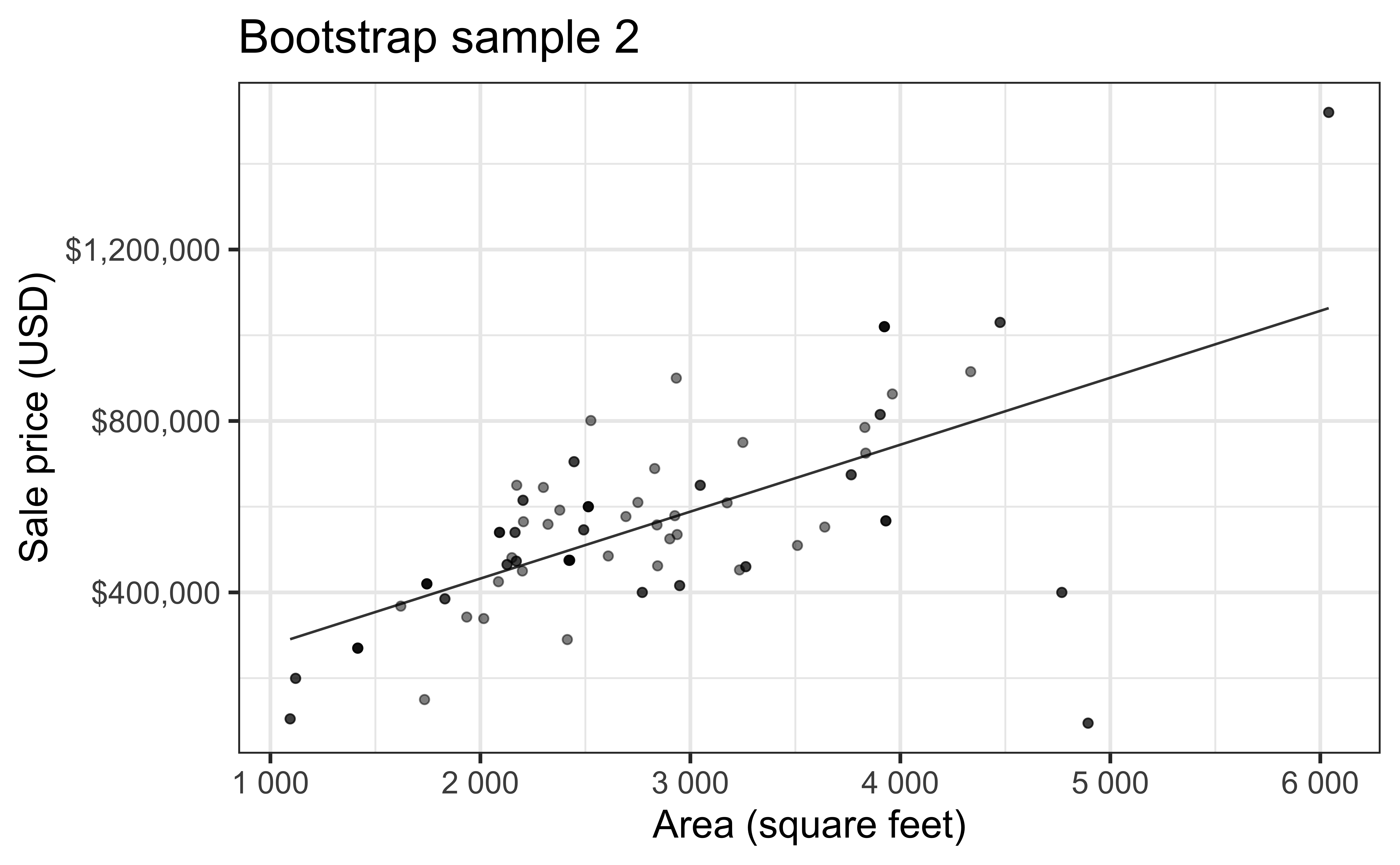
Bootstrap sample 2
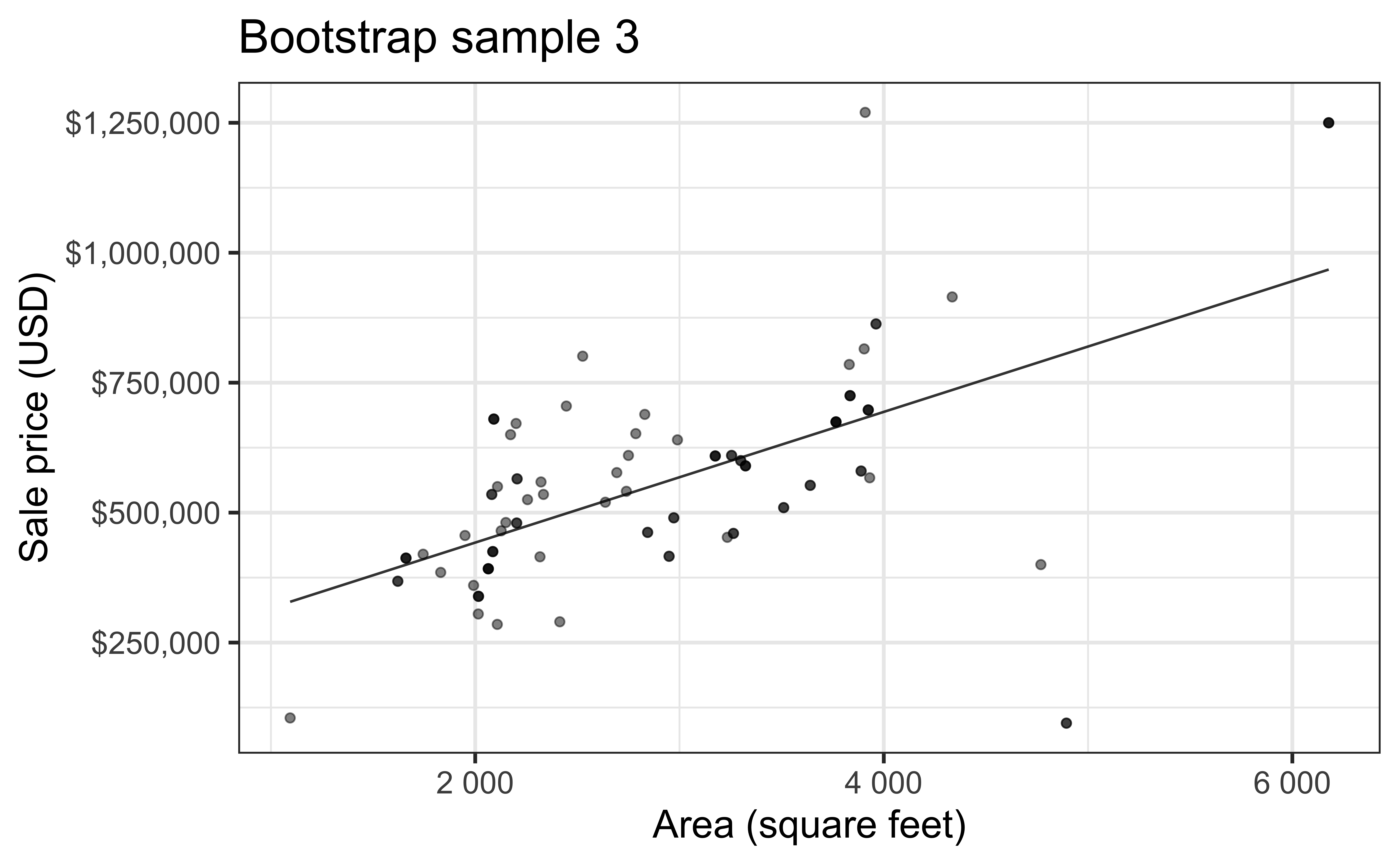
Bootstrap sample 3
Bootstrap sample 4
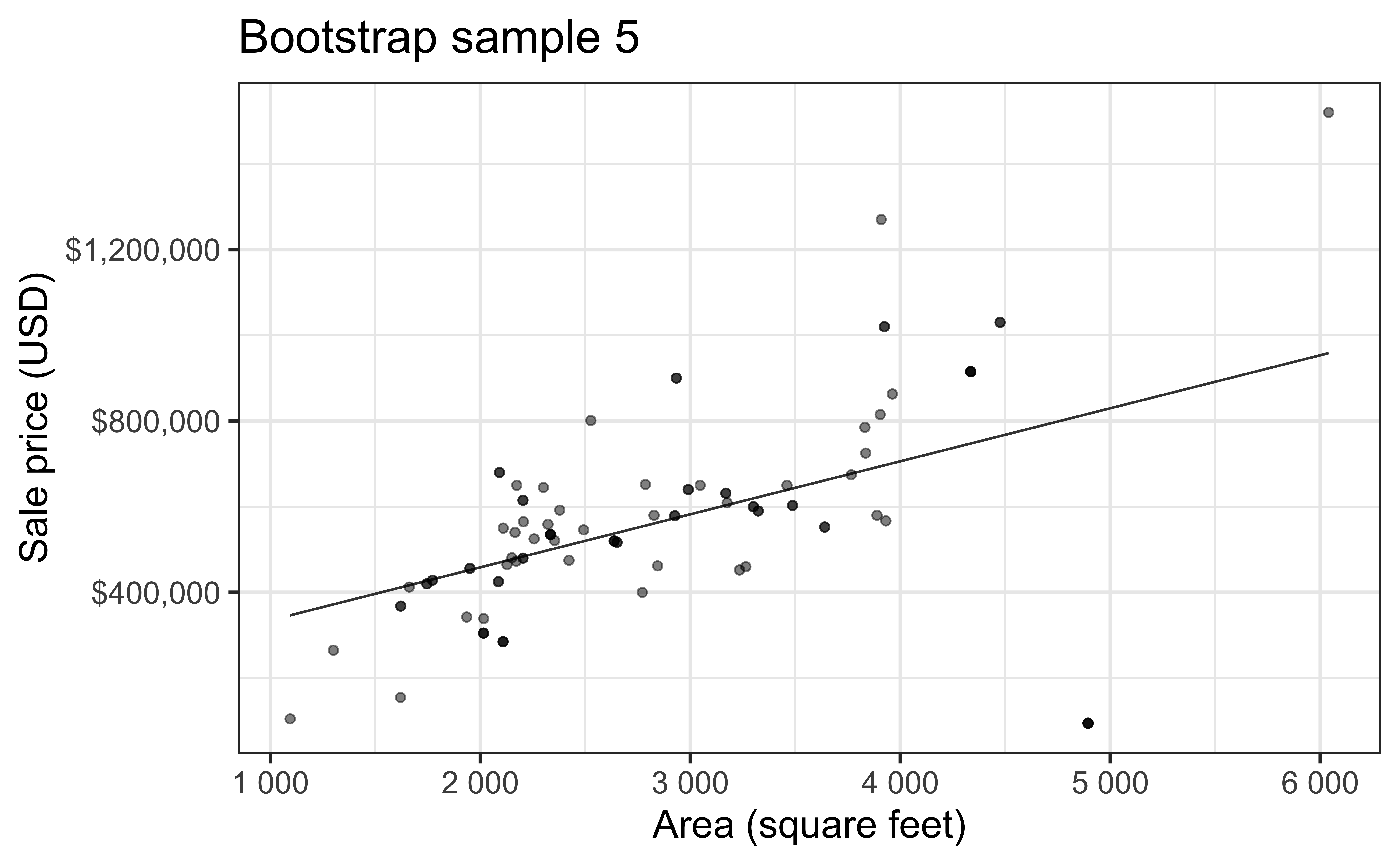
Bootstrap sample 5
so on and so forth…
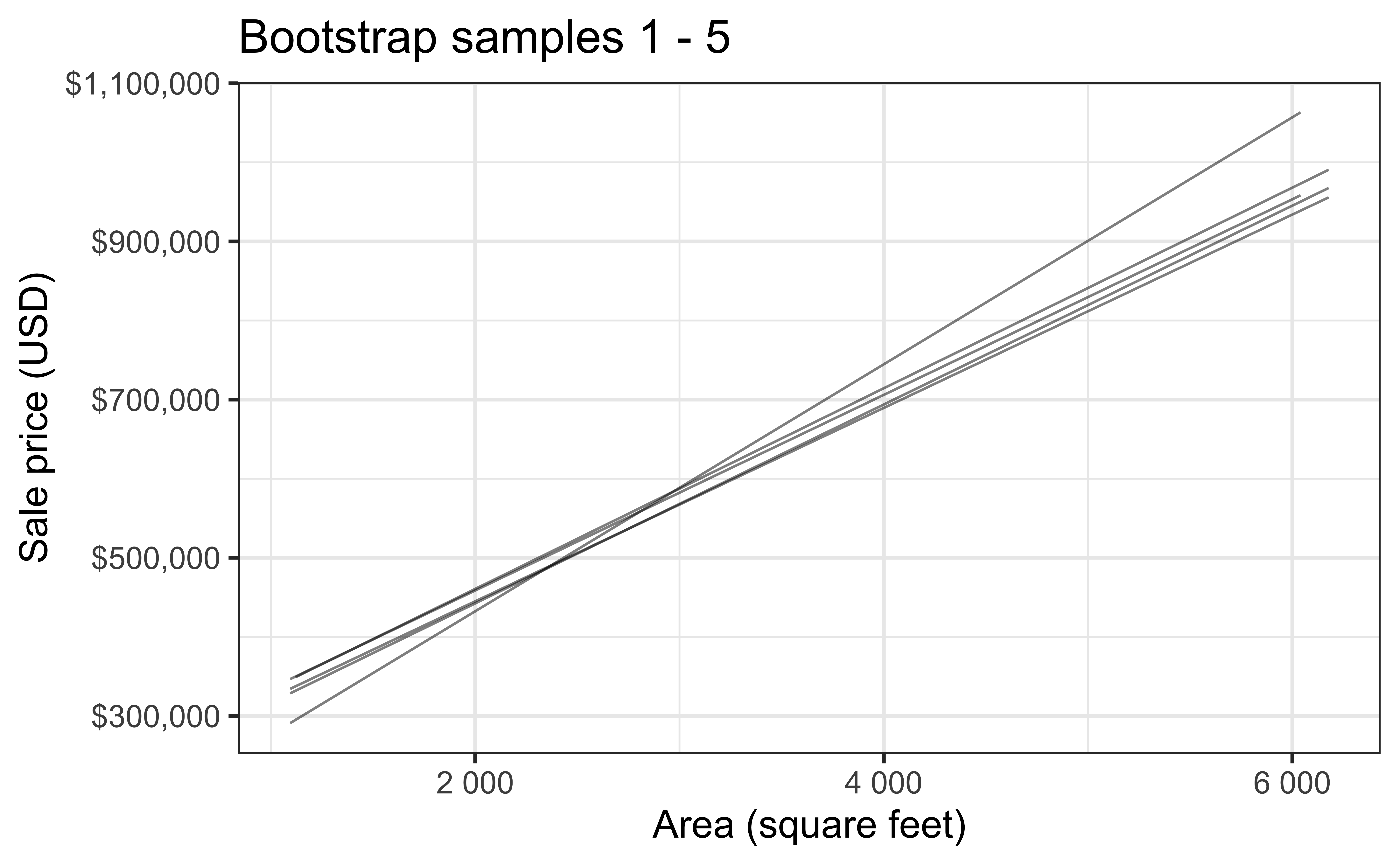
Bootstrap samples 1 - 5
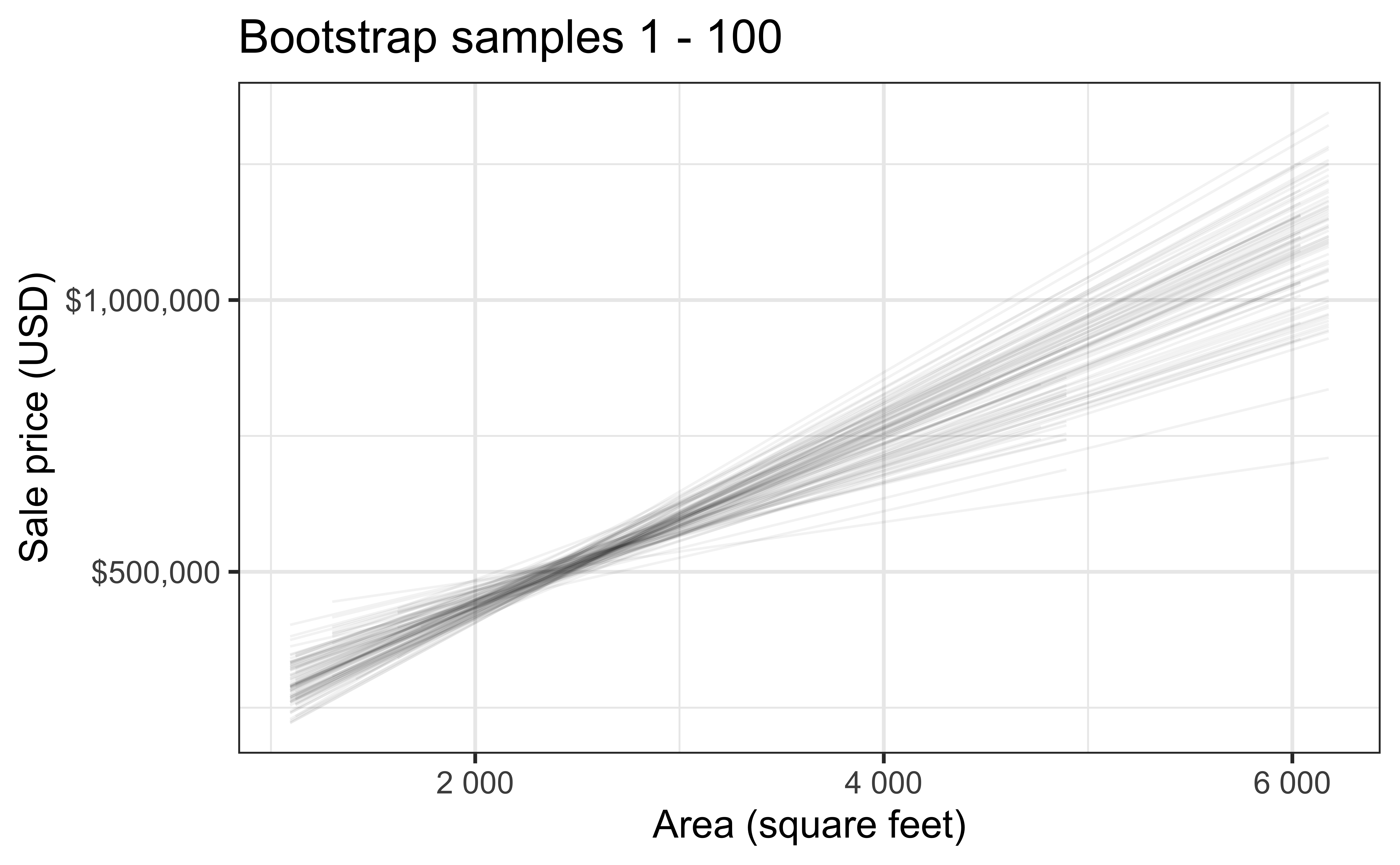
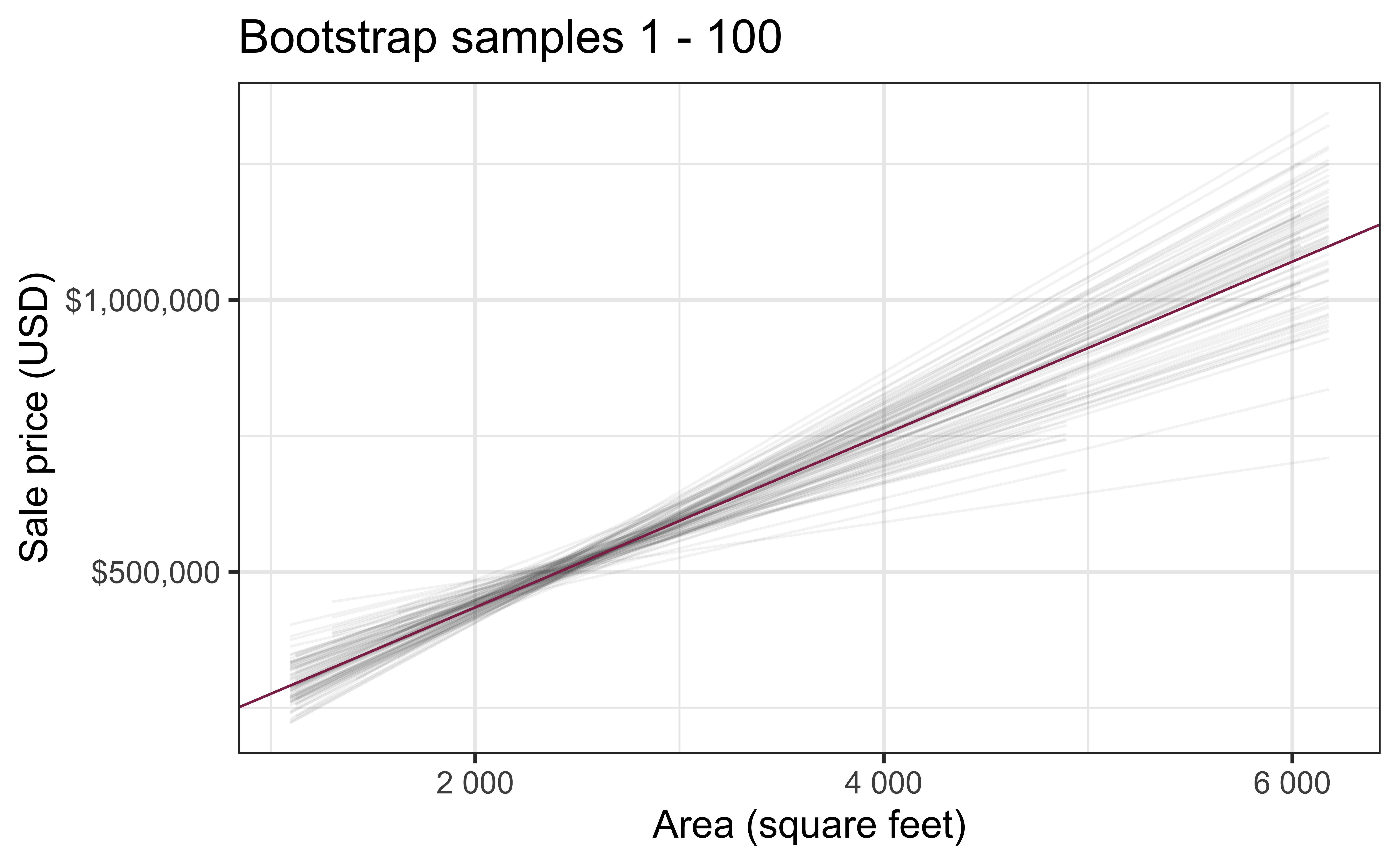
Bootstrap samples 1 - 100
Slopes of bootstrap samples
Fill in the blank: For each additional square foot, the model predicts the sale price of Duke Forest houses to be higher, on average, by $159, plus or minus ___ dollars.
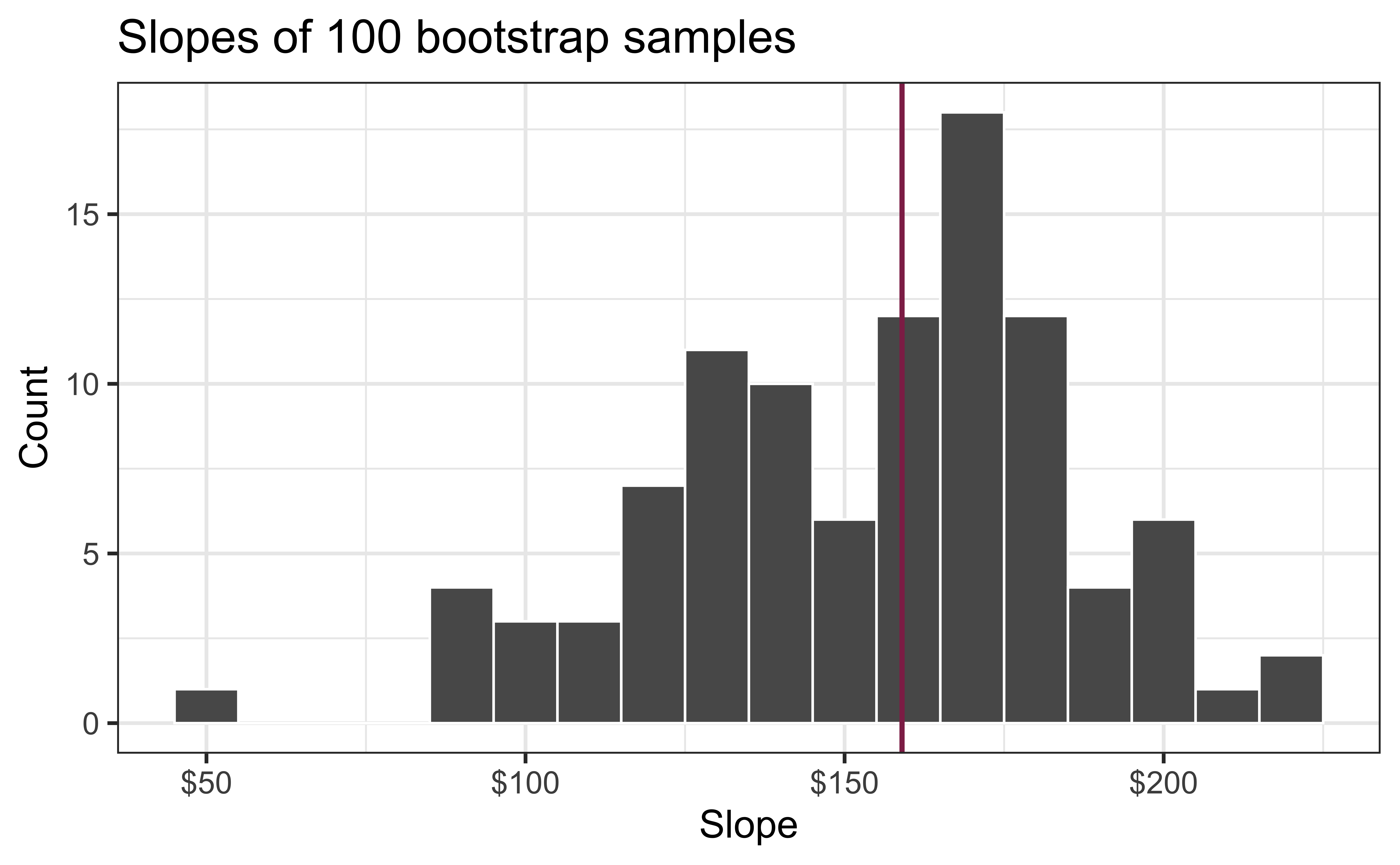
Slopes of bootstrap samples
Fill in the blank: For each additional square foot, we expect the sale price of Duke Forest houses to be higher, on average, by $159, plus or minus ___ dollars.
Confidence level
How confident are you that the true slope is between $0 and $250? How about $150 and $170? How about $90 and $210?
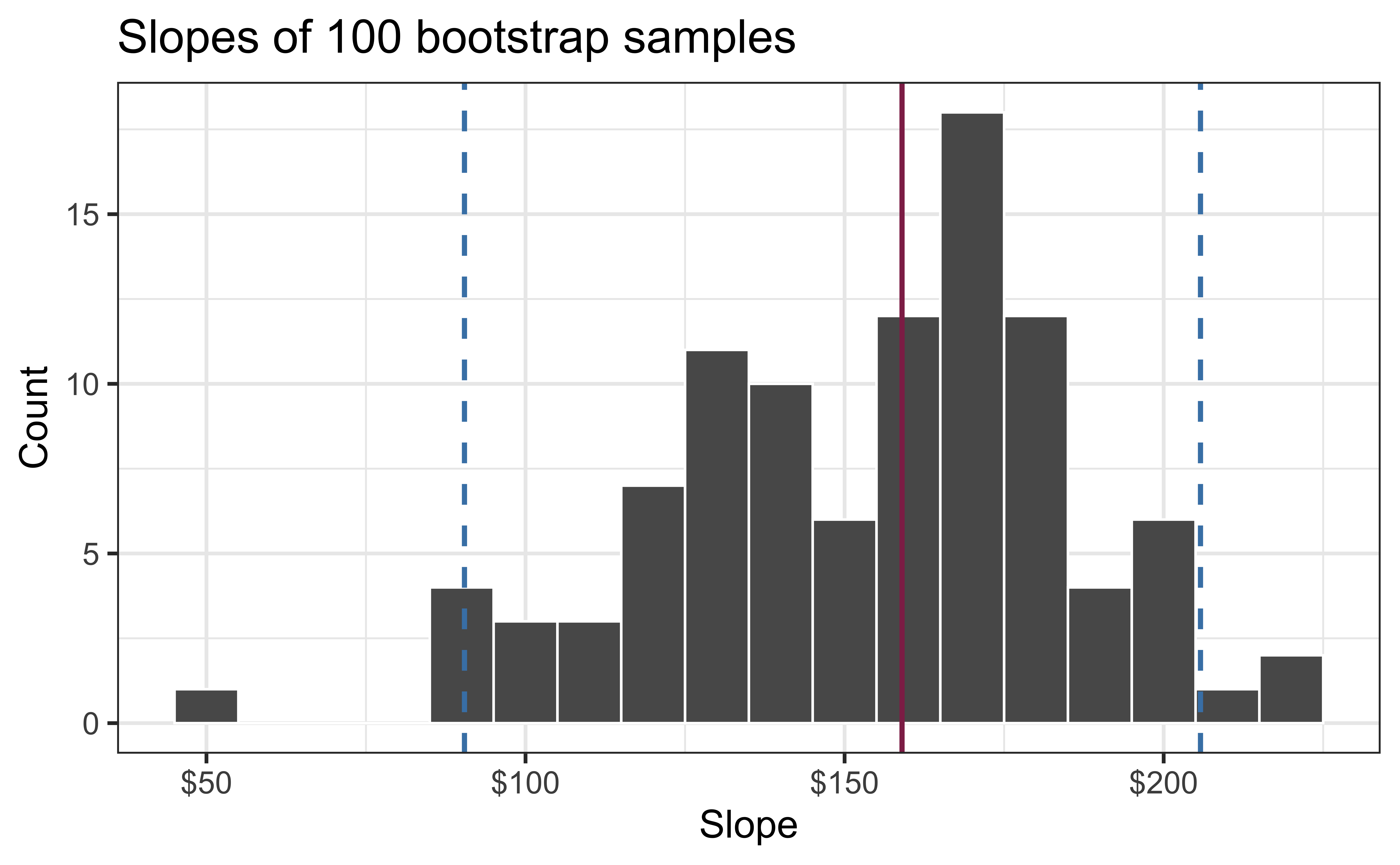
95% confidence interval
A 95% confidence interval is bounded by the middle 95% of the bootstrap distribution
We are 95% confident that for each additional square foot, the model predicts the sale price of Duke Forest houses to be higher, on average, by $90.43 to $205.77.
# A tibble: 2 × 3
  term      lower_ci upper_ci
  <chr>        <dbl>    <dbl>
1 area          92.1     223.
2 intercept -36765.   296528.
Precision vs. accuracy
If we want to be very certain that we capture the population parameter, should we use a wider or a narrower interval? What drawbacks are associated with using a wider interval?
Precision vs. accuracy
How can we get best of both worlds – high precision and high accuracy?
Changing confidence level
How would you modify the following code to calculate a 90% confidence interval? How would you modify it for a 99% confidence interval?
# A tibble: 2 × 3
  term      lower_ci upper_ci
  <chr>        <dbl>    <dbl>
1 area          56.3     226.
2 intercept -61950.   370395.
Recap
Population: Complete set of observations of whatever we are studying, e.g., people, tweets, photographs, etc. (population size = \(N\))
Sample: Subset of the population, ideally random and representative (sample size = \(n\))
Sample statistic \(\ne\) population parameter, but if the sample is good, it can be a good estimate
Statistical inference: Discipline that concerns itself with the development of procedures, methods, and theorems that allow us to extract meaning and information from data that has been generated by stochastic (random) process
We report the estimate with a confidence interval, and the width of this interval depends on the variability of sample statistics from different samples from the population
Since we can’t continue sampling from the population, we bootstrap from the one sample we have to estimate sampling variability